Detailed CODAS Guide
Using quick_adcp.py to process ADCP data
Table of Contents
Introduction
Shipboard ADCP data processing requires several necessary steps. The reality of data (and all the things that can to wrong) make the steps more complicated than one might expect at first. Basic processing of a clean dataset is easy; any problem with the data increases the complexity of the processing.
CODAS (Common Oceanographic Data Access System) is a database designed to store ADCP data and associated information (eg. heading, time, position). The CODAS database is simply a vehicle for storage and organization of the ADCP data while various processing steps are run. “CODAS Processing” refers to the University of Hawaii collection of programs that use the CODAS database to process ADCP data.
CODAS processing steps are designed to be flexible (to cope with different data sources and problems encountered during processing) and automatable (so the basic steps can be run easily with minimal overhead per dataset). Many datasets do not need all of the flexibility available, but since some data streams sporadically fail and some improve over time, there are necessarily many options in CODAS.
quick_adcp.py is a tool to streamline the basic processing steps and provide a uniform naming convention for the various files used in processing. It has various switches that are required and others that are used to specify the kind of data being processed.
This document is designed to introduce the CODAS processing steps run by quick_adcp.py, point to other tools and resources, and help the user understand how to use quick_adcp.py for their particular dataset.
NOTE: Prior to using Univ. Hawaii CODAS processing software, a computer must be set up with the appropriate software. Details of the computer setup are available here.
CODAS processing overview
Here are the basic steps in CODAS processing of a shipboard ADCP dataset. You may have other steps that need to be addressed.
Stage averages on disk (one of these)
load pre-averaged ADCP data
DAS2.48 (RDI’s DOS software created “pingdata files”, usually from a NB150 ADCP).
stage pre-averaged ADCP data on disk
VmDAS (RDI’s Windows software creates “LTA” or “STA” files) Runs on BB, WH, or OS (not NB).
make averages from single-ping data, stage on disk
UHDAS (Univ Hawaii linux acquisition system, can create averages for use with CODAS processing)
VmDAS (RDI’s Windows software creates ENR files that can be converted to a UHDAS-like directory structure (along with supporting ancillary data) and averaged as if they are UHDAS data.
Note
Transect (RDI Windows 3.1 software, usually used with BB, is not supported by CODAS Python processing)
create the database, add all ancillary data to database
scan –look through the times of the data files to see if there are problems with the PC clock or other problems with timestamps; get the time range of the data.
load – load the averages into the database
navigation steps – clean the navigation using a smoothed ocean reference layer; load the clean navigation and adjusted ship speeds into the database.
quality checking and calibration (repeat as necessary)
scale factor – if fixed transducer (NB, BB, or WH) check speed of sound; scale factor calibration may be necessary. Should not be necessary for OS.
heading correction – gross transducer offset, time-dependent heading correction
graphical editing – throw out bad bins, bad profiles, and data below the bottom
accessing data
adcpsect and adcpsect.py (extract ocean velocities with editing flags applied)
getmat and variants (generate matlab files containing most variables: velocity, amplitude, correlation)
temperature and heading (accessing temperature and heading)
Return to TOP
Setting up a Processing Directory
ADCP processing is done in a directory that is created by running
adcptree.py. The processing directory is initialized with a
particular collection of subdirectories and files. Some of those
files are present for all CODAS processing directories, and some are
specific to particular kinds of datasets. The processing directory
should be in a working area of your disk, NOT in the UH programs
directory tree.
Type “adcptree.py for usage, specifically if processing averaged data (LTA, STA, pingdata). Type the following to get more usage information for single-ping processing:
adcptree.py --help
NOTE: Examples for this document were run on a linux machine, with
UH programs rooted at /home/currents/programs.
Processing Strategy
It is important to keep the processing directory relatively free of clutter. If the data are worth using, it is likely that someone will look around in the processing directory for information about how the data were processed and what anomalies were present. Preserving a relatively linear path from the start of processing to the end of processing helps the person later figure out what was done.
Sometimes the best thing to do is simply delete the whole processing directory and start over. It is therefore best to keep original data and processing notes out of the actual processing directory until you are sure you won’t be deleting it for some reason.
We recommend a directory structure like this for adcp processing:
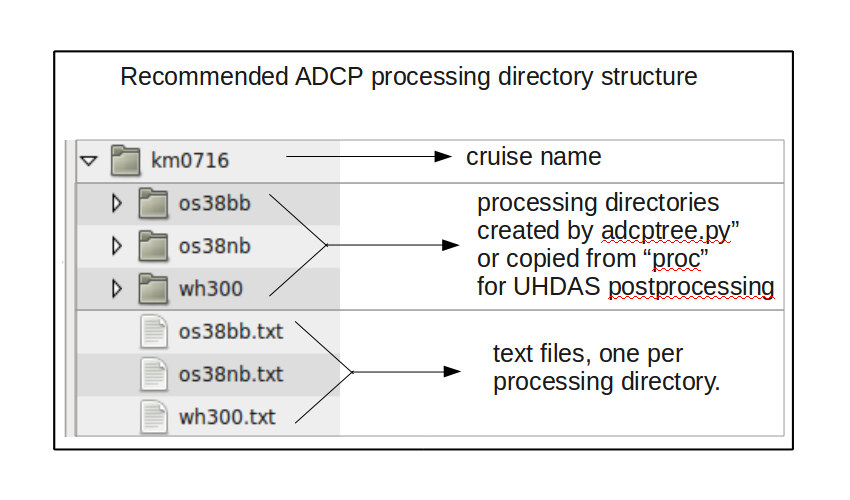
Bearing that in mind, here is one approach to processing strategy
make a directory for the cruise that will hold:
the processing directory
summary notes (metadata file; instrument configuration, dates…)
detailed notes (eg. comments about the data, such as gaps, biases)
instructions (suitable for cut-and-paste for your next attempt)
quality directory for exploration of the data
run “adcptree.py” to make your processing directory
write down the adcptree command you used in a file
name the file something related to the processing directory name
keep the documentation file outside the processing directory until you’re done with it. That makes it easier to redo the steps from scratch without losing the file (if you have to start over)
type the following to see the right prompts for the datatype you have (eg. LTA)
quick_adcp.py --help
type the appropriate help query for quick_adcp.py, eg:
quick_adcp.py --commands lta
proceed to process the data
write down enough of what you do that you can
can use it in 4 months to remind yourself of what to do with the next dataset
can show it to someone else as a tutorial
start over if you need to change processing parameters or made a mistake.
Note
Inside the processing directory is a file called
cruise_info.txt which has the beginning of a reasonable
text file. Start with that; it is already tailored for your
processing directory.
A note about the database name
The CODAS database is actually a collection of binary files whose names are composed of a prefix, a 3-digit number, the suffix “blk”. There is one database directory file (also binary), whose name has the same prefix, and ends in “dir.blk”. Here is an example:
ademo001.blk
ademo002.blk
ademo003.blk
ademo004.blk
ademo005.blk
ademodir.blk
The prefix here, ademo is called the database name. In the control
files used by quick_adcp.py, you will see examples of a relative path
to the database, such as
DBNAME ../adcpdb/ademo
This name is specified when quick_adcp.py is run, and is the prefix for many files. Those files are distinguishable by the directory they are in and the suffix they have.
Note
Anytime a database name is referred to in this document, the
example will use ademo. Anytime the string ademo
is used, it is referring to the database name.
Making the processing directory
Following the instructions in the demo or in the quick_adcp.py help,
use adcptree.py to create a processing directory.
The processing directory is created with the following subdirectories:
The ping directory is the default repository of pingdata files (usually called PINGDATA.* (The data location can be overridden in quick_adcp.py)
The config directory holds UHDAS single-ping processing parameters. It is only relevant if you are going to re-process the data. For post-processing (edit, calibration) it is irrelevant
The scan directory will be used to hold a list of time ranges and time info for each data file. The full time range of the dataset is also stored here
The load directory will be used for loading the data into the database. For pingdata, one executable does this. For all other data types, a two-step process exists:
three sets of files are generated: a pair (suffix bin and cmd) with data for the database, and another set (suffix gps2) with time and position at the end of each averaging period.
load
*.binfiles into the database; stage*.gps2for naigationThe adcpdb directory will contain the database and the configurations used during acquisition
The nav directory will be used for navigation calculations, including smoothed reference layer and plots of same.
The edit directory will be used by dataviewer.py edit mode.
The cal directory will be used for calibration calculations.
cal/rotate (time-dependent heading correction stored here)
cal/watertrk (watertrack calibration and ADCP-GPS offset)
cal/botmtrk (bottom track calibration)
cal/heading (not used by quick_adcp.py)
The contour directory is used to store data suitable for making contour plots (eg. 15 minute averages of 10-20m vertical bins)
The vector directory is used to store coarser averages suitable for vector plots (eg hourly averages of 50m vertical bins)
other directories – These are sort of fossils
The grid directory will be used to grid the data for plotting.
The quality directory contains Matlab scripts for plotting on-station and underway profile statistics; this is a good place to stage your own QC investigations.
The stick directory contains programs to make summary plots of some specific spectral information, treating the data as a time-series (not used by quick_adcp.py)
Return to TOP
UHDAS postprocessing
Note
Under most circumstances, a UHDAS dataset brought back from sea is already processed, and all that remains is manual post-processing (check heading correction, check calibration, edit, document)
Examples for quick_adcp.py processing start here. You should work through the example and become familiar with the postprocessing steps (heading correction, calibration, editing) before attempting to process a single-ping dataset from scratch.
Return to TOP
quick_adcp.py operations
Quick_adcp.py contains quite a bit of documentation about itself.
Running “quick_adcp.py –help” shows how to get help with the usual kinds of datasets. On-line access to that help is here
Note
Always run quick_adcp.py from the root of the processing
directory (the directory created by adcptree.py)
Return to TOP
First pass with quick_adcp.py
Scan
Prior to loading the database, we scan the data files in order to determine whether there are issues with timestamps that need to be addressed. The “Scan” step performs two operations:
list time ranges and perhaps otherinformation about the data files
create a file with the time range of the data
Pingdata are scanned using the executable “scanping”. Go to the PINGDATA demo (Python Processing), and look at the “scan” section for a complete description of the output of “scanping”.
All other data (VmDAS and UHDAS) are scanned by the processing engine (Python). In either case a little standalone program is written and then run. The main point of this step is to get the time range.
If the database name of this example is “ademo”, the following files are written:
ademo.scn (contains timestamp information about the data files)
ademo.tr (a human-readable time range, extracted from ademo.scn)
Note
CODAS time stamps come in two flavors.
year/month/day hour:minute:second (such as 2011/04/17 14:02:32)
zero-based decimal day (i.e. January 1 noon UTC is 0.5, not 1.5)
CODAS database timestamps refer to the end of the ensemble
Return to TOP
Load
averaged data
The “load” step refers to “loading” the data into the database.
Historically (“Pingdata”), the files were loaded into the database with
one executable program. For modern (VmDAS, UHDAS) data, files with
averaged profile information are staged in this directory and then the
ldcodas program reads data and creates the database from those
files.
The averaged profiles are stored in the load directory as pairs of
files (*cmd and *bin), with the cmd files containing
instructions to “ldcodas” and the bin files containing the data.
The *.gps2 files contain times and positions at the end of the
ensembles. Those are used later in the “nav” dirctory.
single-ping data
For singleping data, more configuration information is required, since the raw data do not yet have corrected timestamps or any ancillary data.
Processing UHDAS data entails reading the single-ping ADCP data
(correcting time and adding navigation and attitude), editing the
single pings, averaging the data, and writing the *bin and
*cmd files. Then ldcodas creates the database.
Note
Processing UHDAS data from scratch requires a good grounding in CODAS processing, which can be obtained by working through examples with LTA data or by post-processing a UHDAS dataset.
VmDAS data include three kinds of single-ping data. Although CODAS Python programs can read ENS and ENX data, they may contain timing or other errors, so we use the ENR data. Configuration information is required to properly parse the ancillary data. These are reformed into fake UHDAS data, and then processed as if they were acquired as UHDAS data.
“Pingdata” refers to averaged data acquired by DAS2.48. See this note.
Return to TOP
Checking the database
After any quick_adcp.py step, you may want to check the database to see what changes you have made and to ensure that everything is working as expected. This is not a step run by quick_adcp.py. You can go to another command-line window and run the following command as you work your way through the quick_adcp.py steps:
showdb adcpdb/ademo
The program showdb is ascii menu-driven command-line utility exists
to probe the database and determine what is stored in it. There is no
substitute for this important but old-fashioned program.
The PINGDATA demo (Python Processing) explains showdb in detail, using the original pingdata demo, in which a database was created using two pingdata files. There are various examples of showdb throughout the original pingdata demo instructions.
Note
You can use showdb to check various aspects of the database. For instance, immediately after loading, the database will contain measured velocities, depths, heading, and various configuration information, but the positions will show MAX, i.e. bad values: positions are loaded in a later step.
Return to TOP
Heading Correction
Accurate heading is essential for high-quality ADCP data. An error in heading of X degrees causes an error in the cross-track direction that scales as
error = shipspeed * sin(X).
For a ship travelling at typical cruising speeds, i.e. 5m/s (10kts), a one degree error in heading causes a cross-track error of 10cm/s. Gyros, especially older gyros and especially in low latitudes, can wander significantly, causing completely spurious cross-track errors that manifest as “eddies” in the data.
An example of a few degrees offset is shown deep in the documentation for dataviewer.py. This page jump to it here graphically illustrates the difference an error of 2 degrees degrees makes on a dataset.
Headings can come from a variety of sources, some more accurate than others. Your access to headings depends on a variety of factors
the acquisition system (UHDAS, VmDAS, DAS2.48+ue4, DAS2.48)
- the instruments available on the ship (gyro (serial or synchro),
Ashtech, Seapath, POSMV, various optical gyros)
- the setup of the acquisition system and data feeds (wrong messages?
instrument failed? data recorded elsewhere?)
You need to know (or find out) the sources of heading for your dataset, what is available where (which files contain which information), and what heading source was used for processing. If there is only one heading device, your options are limited. If there are both gyro and some other heading source, you can compare them to see what the differences are in quality and behavior, and either correct the data (if acquired with gyro) to the other source, or (if processed with the other source) possibly make a statement about that instrument’s data quality.
If you have UHDAS data, the strategy is to use gyro data for the
initial conversion from beam to earth coordinates, and correct that
with the 5-minute average of the difference between the gyro and the
other heading device. In older processing, this was done in a batch
mode, rotating the database after the database was created. In newer
UHDAS processing, the heading correction is built into the averages
(*bin and *cmd files) before they are loaded into the database,
and the values used are recorded to disk (cal/rotate/ens_hcorr.ang)
If you have VmDAS data, you may have more than one source for heading,
depending on whether there is a synchro gyro input (Ocean Surveyor only).
Check the N1R`, N2R, and N3R files for heading messages.
If gyro was used as the primary heading device, a time-dependent
heading correction might be computed and be applied to the database.
If you have pingdata, and if ue4 was used, and if there was an ashtech on board, the likely source of heading correction data is extracted from ubprint. After loading the database, the time-dependent heading correction can be examined, (corrected if necessary), and applied to the database.
Notes:
A time-dependent heading correction file can be generated and applied after the first-pass processing is complete.
A constant angle rotation is usually necessary in the second-pass steps
You can use
showdbto examine the correction value (ANCILLARY_2)You can extract the original heading and the total correction presently in the database using lst_hdg (extracts values from
ANCILLARY_2)You can return the heading correction to zero by using the
rotatecommand with a suitably-modified control file.
The rotation step takes place in the cal/rotate directory. If there
is a time-dependent heading correction file, plot the corrections and
make sure you are applying something reasonable to the database.
Return to TOP
Calibration
Bottom track calibration uses bottomtrack data (if there is any) to determine the remaining transducer offset to make the ship track over ground match the track measured by the ADCP.
Watertrack calibration uses the idea that the water velocities should not look any different whether the ship is stopped or moving; turning or going straight. It uses parameters to identify times when a significant acceleration was detected (turn and/or speed change) and calculates what rotation and scale factor would be necessary to make sure the ocean velocity looks the same before and after the acceleration. The calculation is necessarily noisy, and depends on ship behavior. For instance there are probably no watertrack calibration points on a transit, and many on a CTD hydrography cruise or a bathymetric mapping cruise.
The parameters used to detect watertrack calibration points can be tuned, but quick_adcp.py uses particular set and runs the calibration steps during the first pass. These are diagnostics, and give the user some information about further rotation or scaling necessary.
More detail about bottom track and watertrack calibrations are contained in the PINGDATA demo (Python Processing).
A summary of calibration files and the sign convention (plus or minus) is here.
A new calibration calculation has been introduced which is sometimes important: it estimates the horizontal offset between the ADCP transducer and the GPS (used to calculate ship speed). A preliminary page documenting this is here.
Return to TOP
Postprocessing: Determining and Applying Calibrations, and Editing
After you’ve run quick_adcp.py for the first pass, you must edit the averaged data (to remove things like wire interference, data below the bottom, bad profiles), investigate the necessity for further rotation, and decide whether a scale factor is required. This is an iterative process.
If there is a large constant heading error or a time-dependent heading error necessary, it is much harder to edit the data because changes in speed will cause changes in the ocean velocity which may look like errors.
To converge on your final dataset,
Ensure that the time-dependent heading correction (if it exists) as good as possible. If you change the heading correction, rerun quick_adcp.py with
--steps2rerun navsteps:caliblook at
cal/watertrk/guess_xducerxy.outto see what transducer offset was guessed. This value represents the offset remaining between the GPS and the ADCP taking into account the values used so far.
“Signal” values less than 500-1000 probably indicate a poor guess
depending on how the ship is driven, and the cruisetrack for your cruise, offsets less than 5m may not make a big difference.
Apply offsets if one offset is 10m or greater AND the signal is over 1000.
Look at bottomtrack and watertrack calculations, and apply any gross (larger than 1/2 degree) phase correction. If you rotate the database, rerun quick_adcp.py with
--steps2rerun navsteps:calibApply any scale factor if necessary (see below). This “should” be unnecessary for ocean surveyors, but is not unexpected for fixed transducer heads, such as NB150 or WH300.
Go through the data with dataviewer.py edit mode deleting obvious additional bad data. Apply the editing by running quick_adcp.py with these options:
quick_adcp.py --steps2rerun apply_edit:navsteps:calib --auto
repeat until they do not change: check editing; apply calibrations (normally there will be up to 3 passes through the editing, with the last requiring no additional flagging, and up to two applications of phase and scale factor calibration values)
More discussion follows:
Heading Correction:
Heading correction has two components: a time-dependent correction of gyro to Ashtech (POSMV, or Seapath), and a remaining contant offset. See the Heading Correction section for more detail.
To inspect the heading correction used during in an at-sea UHDAS
processing directory, go to the cal/rotate directory and look at
the ens_hcorr.asc file.
If you need to fix the heading correction (eg. there are gaps where no heading correction was applied), you must remove the already-existing heading correction by “unrotating” the database. Then fix the heading correction file, and rotate using the new file. See references to patch_hcorr.py
After the time-dependent correction is made, there may still be a constant offset. Estimates of that value are in the “phase” in watertrack and bottom track calibration files, or from “recip.m” (if there is a reciprocal track available). More details are in the PINGDATA demo (Python Processing) for bottom track and watertrack calibrations.
Scale factor
For a fixed transducer instrument (NB, BB, or WH) a scale factor may be necessary. Check the thermistor temperature to make sure the thermistor is not broken. You may need to fix the speed of sound. It is possible that application of constant scale factor is all that is necessary.
See the PINGDATA demo (Python Processing) discussion about thermistor checking.
Although the Ocean Surveyors should not (in theory) need a scale factor, experience suggests it is not uncommon to need about 1.003-1.005; these are reasonable numbers. If, after editing, the scale factor for an ocean surveyor is still greater than 1%, either there is still a problem with the data (eg. underway bias not edited out) or there is a problem with the instrument. You may need to look at additional datasets or talk to others who have used data from this instrument to try and determine whether you have a problem.
Gautoedit editing
Quick_adcp.py sets up the edit directory for the graphical editing tool, dataviewer.py used in edit mode (docs here ).
This tool was designed to screen data for things like ringing, on-station wire interference, jittery navigation or velocities, and data below the bottom.
A UHDAS at-sea processing directory already has the default dataviewer.py editing parameters applied. You can use showdb to see that this is true.
NOTE: “Flagging data as bad” is mostly a one-way trip: you can add flags to the collection, but if you want to remove them, things get complicated. This page discusses various scenarios.
Use dataviewer.py to look through the database and decide whether any of the missing data should be unflagged, or whether you just need to flag some additional data. Click on the button “do not show dataviewer.py editing” to see what is in the database. Click on “do not show profile flags” to see the original data.
Adding more profile flags
- As you go through dataviewer.py, you can
delete more profiles (time range or individual profiles)
delete rectangles (rzap) or polygons (pzap)
identify the bottom (bottom)
change thresholds to delete more bins or profiles
Note
In general, the dataviewer.py editing summary is:
manually edit (bad profile, delete rectangle or polygon, bottom edit)
modify thresholds if necessary
click “Save Auto Edits”
show next
When you are finished, apply the editing as
quick_adcp.py --steps2rerun apply_edit:navsteps:calib --auto
More detail regarding profile flags (and the underlying application of PROFILE_FLAGS to the database) can be found
in the 1993 PINGDATA demo (revised for Python) describing the application of ascii flag files
profile flags details describing what the actual PROFILE_FLAGS are in the database
check editing and calibrations again
After you think you are done editing, use dataviewer.py to review the data. You should not see any of these signatures in the ocean velocities
transitions between on/off station
ship turn
bias in the direction of ship motion (usually with low PG)
big stripes of missing data at turns or accelerations
If you have sufficient calibration values to tell, your watertrack and bottom track calibrations should have phase within a few tenths of a degree of zero, with all estimates agreeing (mean, median, watertrack and bottom track) also to within a few tenths of a degree (if there are enough points). Scale factor should be within a fraction of a percent of 1.00 (0.997-0.003) and different estimates should agree (mean, median, watertrack and bottom track)
Accessing the Database
See this page for links to ADCP data access tools.
Older CODAS docs
These older files still have relevant details about the inner workings of the CODAS database.
A rejuvinated version of the documentation for processing the 1993 PINGDATA demo in Python contains detail about watertrack and bottomtrack calibrations as well as
showdb. Do not discount this reference.The original CODAS documentation comes as a (PDF file) and contains a lot of detail about the inner workings of the compiled CODAS programs. It was written when Matlab processing was used, and is augmented my the original Matlab 1993 PINGDATA demo instructions.