Underway bias

Underway bias is a general term referring to a velocity signal that

1. is correlated with ship speed, specifically:

   • it is present when the ship is moving
   • it is not obvious when the ship is stopped

2. shows up in the direction of motion, usually a positive anomaly in the direction of motion

3. similar characteristics as when there is a scale factor greater than 1 required, but underway bias is different in that

   • a scale factor will not solve the problem
   • there is usually some vertical structure present in the signal

Examples of underway bias are presented below

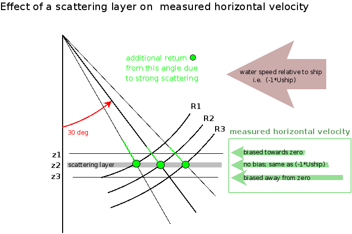
bias due to a scattering layer

This figure shows how sidelobe interference can cause the “S” shape.

This scattering layer signature can be recognized because

• it disappears when the ship stops

• corresponds to a scattering layer (or sharp change in scattering)

  in amplitude (return signal strength)

• the bias has an inverted “S” shape, with bias in the alongtrack direction

  • a lobe of high bias shallower than the layer
  • a lobe of low bias deeper than the layer

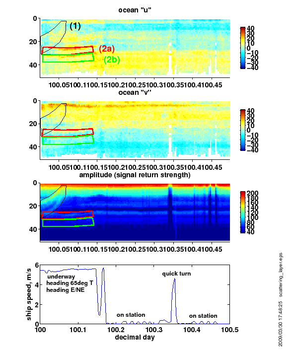
Example #1

The scattering layer might be diurnal migration (labeled “1” in the figure below) or might be persistent in a horizontal layer (labeled “2a” and “2b” in the figure below). In this figure, the ship was steaming E/NE so the bias is most visible in “u”, and disappears when the ship stops. In this example, I would note the time and vertical range where the scattering layer affects velocity, but would not flag it as bad.

Click on the thumbnail to see a larger version.

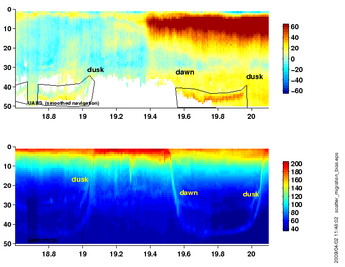
Example #2

In this example, the ship was steaming during most of the period, They stopped twice: once for a brief time around decimal day 18.7 and again just before dday 20. In both cases the range if the instrument increased (common occurrance) and the spurious velocity signal disappeared.

The effect on the velocity is relatively large (maybe 20cm/s) and is obviously correlated with the scatterers migrating down during the day (bin 40-50). During the night, the scatterers left the deep water and went shallower (notice the “reduced range” in the velocity from decimal day 19.1 to 19.5 when the scatterers weren’t there). In this case the data below bin 40 in first half of the dataset should be flagged as bad. The obvious velocity anomaly in the second half should also be flagged as bad.

Top panel: ocean U

Bottom panel: ocean scattering

Click on the thumbnail to see a larger version.

bias due to bad weather

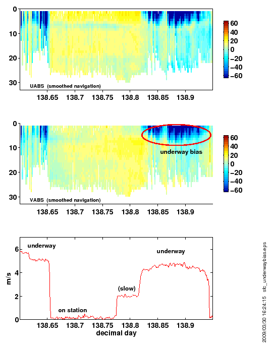
Two examples for a WH300:

1. Enhanced bias in the surface layer. In this case:

• associated with high ship speeds but not on station or slow speed
• bias is negative in U (consistent with ship steaming west, not shown)
• bias is negative in V (consistent with ship steaming south, not shown)

Click on the thumbnail to see a larger version.

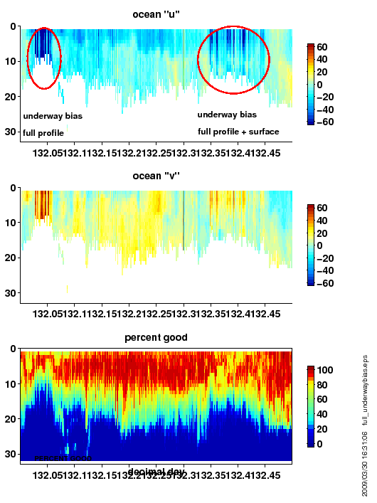
2. Obvious and subtle full-profile bias. In this case

• the ship was steaming north (positive ship V) and west (negative ship U)

• first circled part has:

  • full profiles affected
  • reduced range
  • dramatic: obvious
  • localized

• second circled part has:

  • mixed surface intensification and full profiles affected
  • somewhat reduced range
  • obvious but not as dramatic

• unmarked part:

  • is it biased?

  • WHO KNOWS?

    • look at the other instrument
    • look at velocity in forward dirction
    • look at percent good
    • ??? do your best
    • look at single-ping data (gnarly)

Click on the thumbnail to see a larger version.

bias due to an instrument problem

If the bottoms of profiles show increased velocity in the direction of motion, it could be a sign of an instrument problem. Again, these deep tails are showing a positive anomaly in the direction of motion.

Click on the thumbnail to see a larger version.

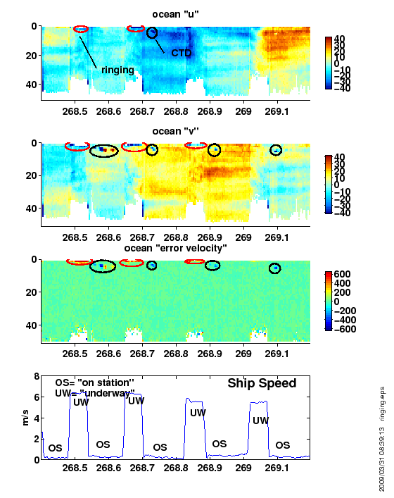
ringing

Ringing comes from measuring the return signal before it has died down. Ringing can be caused by

• blanking interval too short
• reverberation in the transducer well (especially a concern for a transducer well with a window)

Ringing manifests as bias in the direction of motion in the top bins of the data. This is because ringing biases all beams towards zero.

The following figure shows two kinds of shallow scarring. When the ship is underway, surface bins are contaminated by ringing. The ship was travelling to the southwest, so the ringing shows up as negative in U and V. There are also velocity anomalies when the ship is on station. These come from the distortion of the acoustic signature caused by lowering a CTD rosette past one of the beams. The CTD scarring is also visible in error velocity.

Click on the thumbnail to see a larger version.