Understanding Editing (Gautoedit + CODAS)

Gautoedit contribution

Gautoedit (like the original “waterfall plots”) has two kinds of editing: thresholds, and manual. Both append data to ascii files. These files contain the timestamp of the bad profile and information about the flagging.

Gautoedit output

file	file contains ...
abadbin.asc	timestamp and list bins to flag
abadprof.asc	timestamp of whole profile to flag
abottom.asc	bin identified as ‘bottom’

Gautoedit appends flag information to these files. But the information is not transferred to the database until you run

quick_adcp.py --steps2rerun apply_edit  ...

There are two types of editing available:

Threshold Editing

“Threshold editing” refers the adjustment and application of values in the colored boxes along the left side of the gautoedit window. To see how this works, try adjusting “jitter”:

• decrease “jitter”
• click “show now”
• repeat

Any of the colored values on the left can be adjusted and when you clock “show now” it will show you the effect of those thresholds, i.e. what you see (from the gautoedit editing) is what you will get (in the database) if those thresholds are applied.

You MUST click “list to disk” or the flags will not be appended to the ascii files.

Click thumbnail for a larger picture

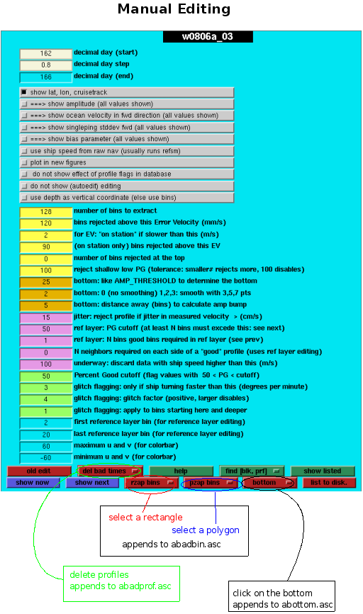
Manual (mouse-driven) Editing

There are basically 4 manual editing buttons:

• del bad times – flag bad profiles
  • click individual profiles; hit <CR> to accept
  • click left and right time range
• rzap bins – rectanglular region slection
• pzap bins – polygon region selection
  • click slowly to mark vertices
  • double-click to finish (connects that vertex to the first)
• bottom – identify bottom (use amplitude to see the bottom)
  • click slowly to identify the bottom
  • don’t guess about bottom blanking; just identify the bottom
  • double click to finish

In all cases, when the tool is finished and the window exits, the flag information is written ascii file.

Click thumbnail for a larger picture

Gautoedit notes

• Only one gautoedit window can be open per matlab session
• As long as the gautoedit window is open, it “remembers” the manual editing that has been done. “Show Now” applies the present thresholds in the boxes when it draws
• The data are extracted to disk when the start time or time step is changed. All other “show now” operations on that collection of data simply read the data, but do noe extract it again.
• Always kill and restart the gautoedit window after you apply the editing to the database. This will make the gautoedit window more in line with the match the flags in the database.
• click the gray bar “do not show autoedit editing” to see what the flags are that com only from the database
• click the gray bar “do not show effect of profile flags in database” to see the data that would otherwise be flagged in the database
• (you can ignore the “bias parameter”; it was experimental)
• (there is a bug when using depth as the vertical coordinate: the flagged rectangles show up in bin space, not meters; sorry)
• You can use the following matlab command to read the data being shown:

data=agetmat('a_');

Remember gautoedit only appends to ascii files; it does not put flags in the database.

Getting flags into the database

The quick_adcp.py step called “–steps2rerun apply_edit” performs several steps. These are performed in the edit/ subdirectory:

1. dbupdate ../adcpdb/dbname abottom.asc

   This step takes any bins identified as the bottom (stored in “abottom.asc”) and identifies them in the database

2. dbupdate ../adcpdb/dbname abadprf.asc

   This step identifies bad profiles in the database by setting the “last good bin” value to -1.

3. badbin ../adcpdb/dbname abadbin.asc

   This step identifies bad bins in the database. A decimal value of 1 is put into “profile_flags” at this stage.

4. set_lgb ../adcpdb/dbname 20

   This step takes the bottom (from #1) and makes flags (decimal flag value of 4) below the bottom. It also masks data close to the bottom if the data are subject to side-lobe contamination (depends on beam angle). The default beam angle is 30 degres. If another number is specified, that is used (eg. “20” in this example)

5. setflags setflags.tmp

   This does two things:

   1. takes the bad profile identifier and and gives every bin in that profile a “bad bin” flag (decimal value of 1)
   2. flags all values with percent good below the specified threshold (usually 30% or 50%) using a decimal value of 2 for the profile flag.

Try using “showdb” to look at a database. The variable “profile_flags” shows the editing status of a given bin or profile. Bins are flagged in the database with a binary bit, depending on why they were flagged. This is a useful way to see whether data have been flagged or not.

binary	decimal	below bottom	percent good	bad bin
000	0
001	1			bad
010	2		bad
011	3		bad	bad
100	4	bad
101	5	bad		bad
110	6	bad	bad
111	7	bad	bad	bad

“Unediting” scenarios

(1) starting over

Example: You have a UHDAS dataset in which too much data were edited out

If you need to start over, you will have to clear all profile flags, remove ascii files associated with editing, and do the editing from scratch. If all you need to do is add flags, just run gautoedit and remove the offending data (i.e. add flags to the existing ones). Here are three examples when you might need to return the flags to zero and start over

• At-sea WH300 data were collected at 2-minute averages, but the default jitter threshold is for smoother data than that. The data in gautoedit will show lots of little white stripes where profiles were thrown out by the jitter criterion that was too low for this dataset
• The gyro was replaced without any change in calibration and the headings are off by several degrees, so profiles at acceleration points (stop/start or turn) are flagged as bad because of the jitter criterion.
• You are training someone else to process ADCP data and they flagged way too many things as bad. You do not need to redo all their processing, just the editing

To start over with editing:

• go to the edit directory
• remove all *.asc files
• copy setflags.tmp to clearflags.tmp
• edit clearflags.tmp as shown below
• run “setflags clearflags.tmp”
• start editing. Be sure to “list” before moving to “next”

original (setflags.tmp)             new (clearflags.tmp)
---------------------------         ---------------------------
dbname:     ../adcpdb/a_demo         dbname:     ../adcpdb/a_demo
pg_min:      50                      pg_min:      50
set_range_bit                        clear_all_bits
time_ranges:                         clear_range
all                                  time_ranges:
                                     all

(2) change percent good

You can change the percent good used by quick_adcp.py (eg. change to 30 instead of 50) by specifying –pgmin 30 but you must do it every time you call quick_adcp.py. Otherwise it will revert to the default.

To change percent good once,

• go to the edit directory
• do not remove any files
• copy setflags.tmp to setflags30.tmp
• edit setflags30.tmp as shown below
• run “setflags setflags30.tmp”

original (setflags.tmp)             new (setflags30.tmp)
---------------------------         ---------------------------
dbname:     ../adcpdb/a_demo         dbname:     ../adcpdb/a_demo
pg_min:      50                      pg_min:      30
time_ranges:                         time_ranges:
all                                  all

Then run

quick_adcp.py --yearbase YYYY --steps2rerun apply_edit --pgmin 30 --auto

(3) Workhorse: (bugfix) recover a few deep bins

“We” (a vigilant user) discovered that bottom blanking was hardwired for 30deg, which is not correct for most Workhorse instruments. This bug only affects data collected when the bottom was in range. Data processed with code prior to May 1, 2009 will have had 15% of the range flagged near the bottom (cos(30deg)), but if the instrument has 20deg beams, the flagging should have been more like 5% (cos(20deg)).

To recover the range 85%-95% of the water column depth from such a dataset

• make sure your executable “set_lgb” accepts an argument for beam angle
• if it does not, follow these instructions to install new programs.
• go to the edit directory
• remove all *.asc files
• copy setflags.tmp to clearflags.tmp
• edit clearflags.tmp as shown below
• run “setflags clearflags.tmp”

original (setflags.tmp)             new (clearflags.tmp)
---------------------------         ---------------------------
dbname:     ../adcpdb/a_demo         dbname:     ../adcpdb/a_demo
pg_min:      50                      pg_min:      50
set_range_bit                        clear_all_bits
time_ranges:                         clear_range
all                                  time_ranges:
                                     all

Now you have a dataset with PG<50 flagged as bad.

• edit astup.m and add the following line to the bottom

  config.beamangle = 20;

Then run

quick_adcp.py --yearbase YYYY --steps2rerun apply_edit --auto

(4) during a gautoedit session, too much was flagged

Example

• “list to disk” was clicked with the wrong thresholds and to much was flagged
• the mouse slipped and the manual (graphical) editing took out too much

In this case the flag information has been appended to the ascii files but they have not been put into the database.

Recommended procedure:

• figure out (in the three files) which lines are the flags that you changed your mind about.
• open the file in an editor and take out those lines
• apply the editing you have done so far

quick_adcp.py --yearbase YYYY --steps2rerun apply_edit --auto

• quit gautoedit and start again.

Now gautoedit is consistent with the database.