4.4. Calculating Ocean velocity from ADCP data
This is a sparsely-annotated collection of figures leading the viewer through the transformation from acoustic ping to ocean velocities.
Acoustic Doppler Current Profiler
Sound is transmitted out each beam at a known frequency.

Acoustic Doppler Current Profiler
Sound returns along each beam, with its frequency changed (Doppler shift) due to water velocity it encounters.
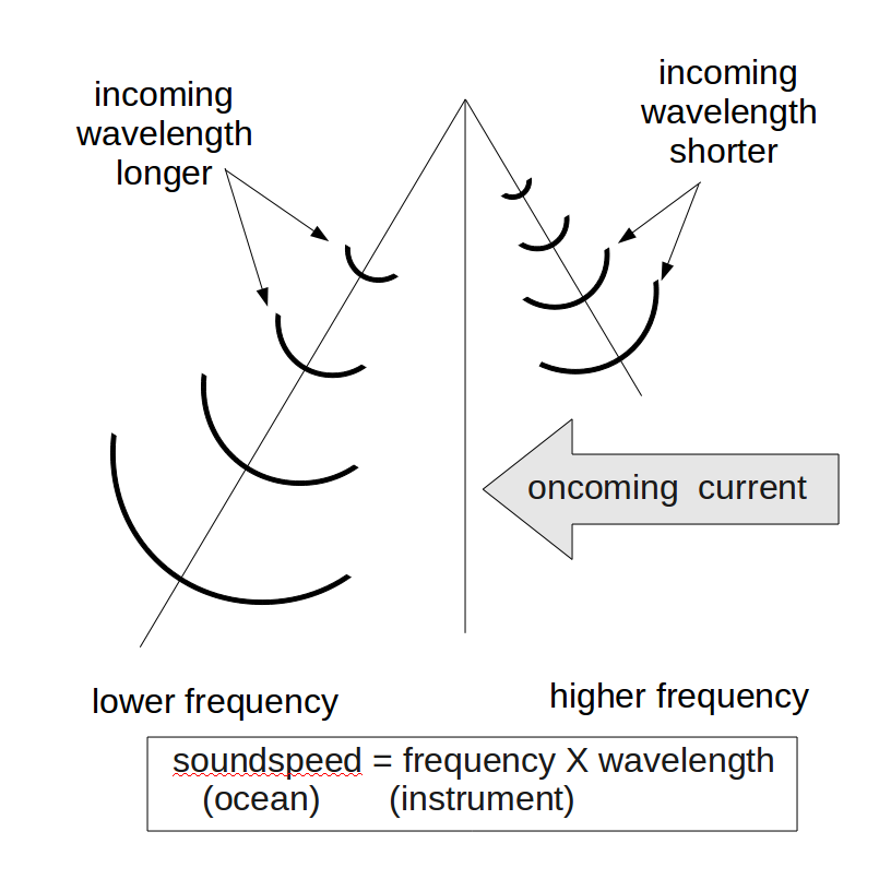
Acoustic Doppler Current Profiler
These profiles are of beam velocity.

The following illustrations go through the steps of transforming from beam coordinates to earth coordinates (East, North, Up)
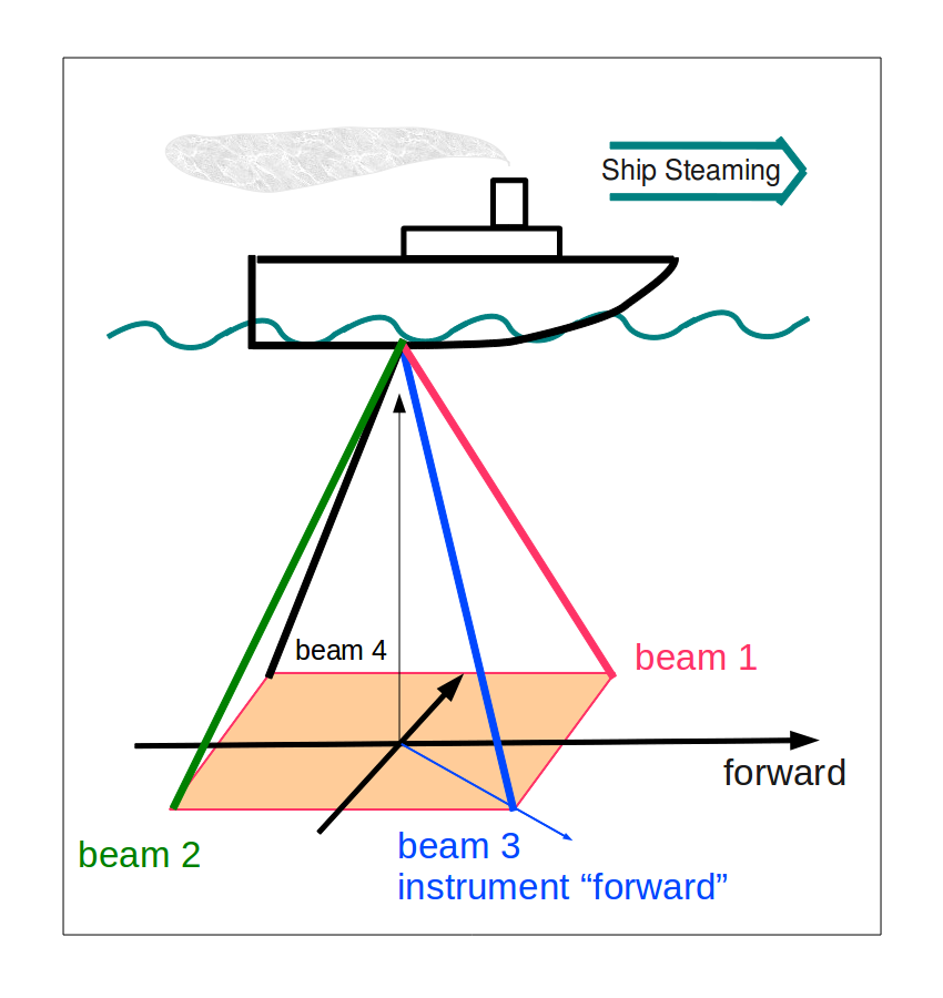
From a bird’s-eye view, the four beams are spread out at 90degrees around a circle. The beam numbered 3 is arbitrarily assigned as the instrument’s “forward” direction, and is often set at 45deg starboard of the ship’s bow.

Switching to a side view, the ship’s coordinate system is “forward” and “port”, and “up”.

Now the four beams are shown. The beams are usually each angled at 20deg or 30deg from the vertical.
Here are both coordinate systems together:

Now we take one pair of opposite beams and look at the velocity past them. The velocity past the the beams is often dominated by the ship steaming.

The two pairs of beams form two vertical planes at 90deg to each other.

Each beam can only measure the velocity along the beam. Like a telescope with a very arrow focus, it can only see things along its line of sight (towards the instrument, or away from the instrument, but only along the beam)

A pair of beams describes a plane, but so does any other pair of independent vectors on that plane. The hands of an analog clock can say 4:30 or they can say 3:00, but both are on the clock face. We transform the pair of beam velocities into a consistent horizontal and vertical pair.

This is does for both pairs of beams.
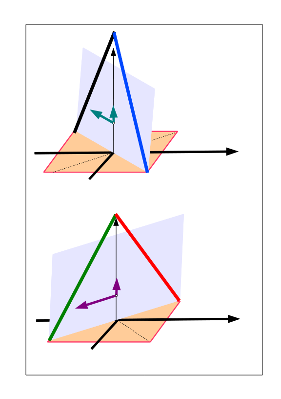
The two horizontal components are now in instrument coordinates. The average of the two vertical components is the ‘vertical velocity’, the difference of the two vertical components is called the ‘error velocity’, and is used as a measure of consistency. A high error velocity indicates the four beams were not measuring the same slab of water.

Note
The vertical velocity from shipboard ADCPs mostly measures the ship bobbing up and down or the vertical tilt of the transducer (if the ship is underway). Vertical velocity from shipboard ADCP may be a useful diagnostic, but does not indicate a vertical ocean velocity.
Rotation of the instrument coordinates by the angle of the “forward” beam to the bow transforms the measurements to ship coordinates.

Rotation of the ship coordinates by the heading of the ship transforms the measurements to earth coordinates.

This figure combines the earlier transformations to show what is required for each step. This takes us from beam coordinates to earth coordinates, but the measurement is still referenced to the ship. The ship is moving. The next step is to take out the motion of the ship.

If there were no ocean velocity, a ship steaming east would result in a measured velocity to the west, i.e. ship and measured velocity have the same value but opposite sign. If there were an ocean velocity it would be changing the ship’s speed by a little bit.

Now the pieces are summarized again.
