2.8.11.1. 1 “PINGDATA Demo” (1993): now with Python Processing
The original version of this document with more detail, but using Matlab programs, is accessible here
This document reworks the original description of CODAS processing
for a 1993 PINGDATA dataset, using CODAS (compiled) binaries and Python.
In modern processing, these steps re usually run using quick_adcp.py,
but the point of this document is to illustrate with some detail, the same
steps, run manually. In particular, this is where to find details
about showdb, bottom track, and watertrack calibrations.
The original CODAS manual
is another source of
detailed information about how the CODAS database works.
Table of Contents
2.8.11.2. 2 PINGDATA DEMO OVERVIEW
Return to TOP
CODAS processing of shipboard ADCP data is a complicated task. Once you are familiar with it, you may find that you do not need all of it’s flexibility. However, since some data streams sporadically fail and some improve over time, there are many options in CODAS. This demo provides a detailed tutorial covering most of the steps one might want to apply to this example PINGDATA dataset.
Here are the basic highlights of processing a shipboard adcp dataset. This can be regarded as an overview when you go through the demo. You may have other steps that need to be addressed.
create the basic ashtech-corrected database
scan
scanping scan.cnt: look at times, beam stats in pingdata.load
loadping loadping: (skip some headers?) create database.navigation steps
ubprint ubprint: get positions and ashtech corr from user buffer. (PINGDATA only)
adcpsect as_nav: get measured u,v.
refabs refabs.cnt: apply reference layer velocity (ocean + ship) from measured velocities.
smoothr smoothr.cnt: Smooth the ocean reference layer velocity and get smoothed positions (nav) from that process.
putnav putnav.cnt: Apply the new smoothed position to the database.heading correction
rotate rotate.cnt: apply ashtech heading correction, if available.
Calibrations:
bottom track
watertrack
apply further calibrations if necessary
Do Graphical (Python) Editing
Look especially for
CTD wire interference
unaccountable jitter rendering a profile bad
seeing the bottom when BT was off
quick_adcp.py --steps2rerun apply_editruns these steps:
badbin ../adcpdb/aship *.asc (if relevant)
dbupdate ../adcpdb/aship badprf.asc (if relevant)
dbupdate ../adcpdb/aship bottom.asc (if relevant)
set_lgb ../adcpdb/aship (required, penultimate)
setflags setflags.cnt (ultimate)
- Apply final rotation using the best guess of phase and amp from cal steps.
(make sure you don’t apply the ashtech correction twice!!)
NOTE:
Any time you alter the database you must run the nav steps again!!! (i.e. adcpsect; refabs; smoothr; putnav) because you’ve changed the data which go into calculating the reference layer.
Note
Notation: In this document
commands to be run in the terminal are not prefixed. Shell results or comments are prefixed with with ‘#’
the simple editor “pico” is used to indicate you are supposed to edit a file
2.8.11.3. 3 SETTING UP
Return to TOP
Your PATH and PYTHONPATH myst be set correctly
(see installation instructions).
Then run adcptree.py to make a new processing directory.
Running adcptree.py occurs with all datatypes and is not specific to
PINGDATA files.
The first argument is the name of the new processing directory that
will be created (usually a cruise ID or instrument name). Here we use
pingdemo. The second argument specifies the data type
(default is “pingdata”, so is unnecesasry in this example)
adcptree.py pingdemo

#Done.

cd pingdemo
ls

#
# adcpdb/ contour/   grid/    nav/         ping/   scan/
# cal/    edit/      load/    quality/    stick/   vector/
These directories are used as follows:
change working directory into this location
run the appropriate steps
change directories back to root processing directory (
pingdemo)
ping/default location for PINGDATA filesscan/stores time range and info about data filesload/staging to load the data into the database.adcpdb/contains the database (and producer definition file for PINGDATA)edit/editing stagecal/calibration calculationsbotmtrk/bottom track calibrationwatertrk/watertrack calibrationrotate/heading correction and rotationheading/(obsolete)
nav/navigation calculationsgrid/store time grids here for data extraction (timegrid, llgrid)contour/extract higher-resolution data here (for contour plots)vector/extract longer+deeper averaged data here (for vector plots)quality/(obsolete) on-station and underway profile statistics.stick/(obsolete) was used for tide analysis
Now copy the raw pingdata files to the ping subdirectory.
cd ping
cp -p /home/noio/programs/qpy_demos/pingdata/ping_demo/pingdata.* .
cd ..
2.8.11.4. 4 PART I: FILL THE DATABASE
2.8.11.4.1. 4.1 SCANNING
Return to TOP
This is the scan step in quick_adcp.py. This step is run
for any data type, but the details of the output are specific
to the data type. This discussion is about PINGDATA output.
Work is done in the scan/ directory:
cd scan
Prior to loading the database, we scan the pingdata files in order to:
check for readability
Any warnings about bad headers alert us to sections that should not be loaded into the database. These are probably due to data recording errors. We have no choice but to omit such profiles during loading.
check the profile times
Since acquisition PC clocks may not be too accurate due to a bad initial setting or drift, it is important to correct the profile times so they can be properly matched to the navigation data. The best time correction can be done during the loading stage. The scanning output will provide a list of profile times. If the user buffer provides satellite times, this step can also be used to pull out this information from the user buffer to help estimate the error and drift in the PC clock, if any. If the user buffer does not contain satellite times, one can also rely on other means (ship log, external navigation file) to come up with the time correction.
ls

#
# clkrate.m    ub_1020.def   ub_1281.def   ub_1920.def  ub_720.def
# scanping.cnt ub_1280.def   ub_1320.def   ub_2240.def

ls ../ping/pingdata.* >> scanping.cnt
pico scanping.cnt
We need to specify the OUTPUT_FILE: (any name will do; we suggest using a .scn extension as a convention). If SHORT_FORM: is set to “no”, the output file will display a list of variables recorded under each header. If you already know what these are, you may prefer to set it to “yes” for brevity’s sake.
The next 3 parameters deal with the user buffer. If the user buffer has been used to record satellite times, then the information can be used to establish accuracy of the ensemble times.
If the UH user-exit program was used, then the user buffer can be any one of the numeric types (1920 for version 4 ue4.exe with direct ASHTECH support; 720, 2240 for version 3 ue3.exe; 1281, etc. from the older version mag2.exe). If you don’t know what kind of user buffer type your data were collected with, use “SHORT_FORM: no” in scanping.cnt and look for “USER_BUFFER” in the .scn file.
For this demo, note that UB_OUTPUT_FILE: is set to “none”, because scanping will go ahead and calculate the PC-fix time and put this as the last column in the main OUTPUT_FILE:.
If another user-exit program was used, it may generate some ASCII user-buffer, which may have some form of the satellite times. That can also be used. In this case, specify a UB_OUTPUT_FILE: name and set USER_BUFFER_TYPE to “ascii”.
Non-ASCII user buffers, including the UH types, are parsed by providing a structure definition file. This is what the UB_DEFINITION: parameter specifies. Detailed instructions for constructing such a file are pointed to in the CODAS MANUAL. The example *.def files in the directory also provide some starting point. If you want scanping to attempt to parse a non-UH, non-ASCII user buffer, try to construct such a file, set the USER_BUFFER_TYPE to “other”, and specify a UB_OUTPUT_FILE: name.
scanping scanping.cnt

#  Stripping comments from control file
#
#   OUTPUT_FILE: aship.scn
#   SHORT_FORM: no
#   UB_OUTPUT_FILE: none
#   USER_BUFFER_TYPE: 720
#   UB_DEFINITION: ub_720.def
#
#
#   PINGDATA_FILES:
#   DATA FILE NAME ../ping/pingdata.000
#
#   Header 1
#   Header 2
#   .
#   .
#   .
#   Header 294
#
#   END OF FILE: ../ping/pingdata.000
#
#
#   DATA FILE NAME ../ping/pingdata.001
#
#   Header 1
#   Header 2
#   .
#   .
#   .
#   Header 286
#
#   END OF FILE: ../ping/pingdata.001
#

ls

#  aship.scn clkrate.m     ub_1020.def    ub_1281.def    ub_2240.def
#  cleanscn  scanping.cnt  ub_1280.def    ub_1320.def    ub_720.def


cat aship.scn
We normally check for 4 things:
- Any warnings about bad headers? Search for “WARNING:”.
None for our demo; if there were, we’ll need to skip them during the loading stage.
For UH-type user buffers, the pc-fix time column shows how many seconds difference there was between the PC and satellite clocks. This does not detect errors in the date.
In version 3 ue3.exe and later, this should never exceed +/- n, where n is the max_dt_difference specified in the ue3.cnf file during data acquisition (assuming that the correct_clock option was enabled). This would indicate that the program did its job of resetting the PC clock to the satellite time whenever it drifted more than max_dt_difference seconds.
For our demo, it looks like the program did its job: the last column is never more than 2 seconds in either direction.
The interval (min:sec) column gives us the difference between profile times.
One would expect that it should be within a second of the sampling interval. When that is not the case, it indicates an ADCP recording gap–either instrument failure, disk full, or momentary interruptions to change some configuration setting (turning bottom tracking off/on, etc.).
For our demo, this column clues us in on the noisy ensembles we observed from the preliminary plots: they (headers 7, 8, 75, 76, 290, 291 under pingdata.000) are only 2 or 3 seconds long, instead of 5 minutes! This is caused by an early version of the clock resetting scheme in ue3; when it set the clock back at the start of an ensemble, the DAS promptly ended the ensemble. This is not a problem for current versions of ue3. We will not load those too-short ensembles.
Was bottom tracking used at any time? Search for “bottom” or “ON” and “OFF”.
INFORMATION:
For more information on types of time correction problems and clkrate.m,
see the original pingdata matlab demo
and the original CODAS Manual.
There are other useful pieces of information in this file:
Are the profile times reasonable?
Header breaks can signal interruptions for the purpose of changing configurations or resetting the ADCP time. (Note that for the demo, there is a header for every profile because the raw data did not come directly from the ADCP recording disk, but through a serial connection that allows the user-exit program to pass a copy of the ensemble data to another machine. This feature attaches the header to each ensemble).
For each input file the last entry in the scanping output file is a table giving a statistical summary of the “beam statistics”.
This gives a general indication of the depth range achieved in that file and, more importantly, shows whether all four beams were performing similarly. Differences can provide an early warning of beam failure.
When finished, change back to processing directory:
cd ..
2.8.11.4.2. 4.2 LOADING
Return to TOP
This is the load step in quick_adcp.py. This step occurs
for all data types, but the details here apply only to PINGDATA.
Work is done in the load/ directory:
cd load
Prior to loading, we need to make the producer definition file. This file identifies the producer of the dataset by country, institution, platform, and instrument. It lists the variables to be recorded, their types, and frequency of storage, etc. Finally, it defines the structures for any STRUCT-type variables loaded. Details about this file are given elsewhere.
cd ../adcpdb
cp adcp720.def aship.def
pico aship.def
The *.def files in the adcpdb/ directory are already set up for the R/V Moana Wave shipboard ADCP recording UH-type user buffers. Other producers may edit them to specify the proper PRODUCER_ID (it is not essential, as NODC no longer uses these codes), and review the variables listed (mostly a matter of switching between UNUSED and PROFILE_VAR if a different set of recorded variables are selected–this is rarely the case) and with regard to the user buffer structure definition. If the user buffer is ASCII, change the value_type field from ‘STRUCT’ to ‘CHAR’ and delete the USER_BUFFER structure definition. If it is non-UH and non-ASCII, paste in the appropriate structure definition.
Next we prepare the loadping control file.
cd ../load
ls
# loadping.cnt
ls ../ping/pingdata.\* >> loadping.cnt
pico loadping.cnt
Aside from attaching the list of raw pingdata files, we need to specify the DATABASE_NAME (no more than 5 chars. to satisfy PC-DOS conventions), the DEFINITION_FILE: we set up from above, and an OUTPUT_FILE: name for logging.
The next 4 parameters define how to break the raw data up into CODAS block files. Note that each block file requires some overhead disk space (rather minimal), so it is not a good idea to generate more than is necessary. The loading program will ALWAYS start a new block file when it detects that the instrument configuration has changed, because instrument configuration is constant over a given block file. The 4 parameters in the control file allow the user to define further conditions that can break up the data into more block files. MAX_BLOCK_PROFILES: can be used to limit block file size so that each one can be accommodated on a floppy disk, for example. NEW_BLOCK_AT_FILE? set to “yes” makes it easier to associate a given block file with the pingdata file it came from. (An example of a case where a “no” makes sense is where data are recorded onto 360K floppies, and the DAS records one big pingdata.000 file and one small pingdata.001 file on each.) The NEW_BLOCK_AT_HEADER? is necessarily a “no” for the demo, where each ensemble has a header, and generally “no”, since the foregoing criteria, plus the NEW_BLOCK_TIME_GAP(min): are sufficient for most purposes. A “yes” may be used occasionally for tracking down particularly troublesome datasets. The NEW_BLOCK_TIME_GAP(min): is also useful. A time interval of 30 minutes or more is often a sign of trouble (a time correction overlooked, for example) or could actually be a couple of days in port and a transition from one cruise to another. Breaking the database at those points can make it easier to track/correct such problems at a later stage.
Following each PINGDATA_FILES: filename can be a list of options to either skip some sections during loading or apply a time correction as the data are loaded, as determined from the scanning stage. An ‘end’ is required to terminate this list, even where it is empty.
For our demo, we do not need any time corrections, just some skips over the too-short ensembles we have found from the .scn file.
Now we load the data:
loadping loadping.cnt

 #  Stripping comments from control file
 #
 #  -------------- start ----------------
 #  pass 1: checking the control file.
 #  .
 #  .
 #  .
 #  pass 2: loading pingdata file into database.
 #
 #  Data file name: ../ping/pingdata.000
 #  % OPTIONS:
 #  % =======
 #  % skip_header_range:
 #  % skip_header_range:
 #  % skip_header_range:
 #  % =======
 #
 #  Header 1
 #  Header 2
 #  Header 3
 #  Header 4
 #  Header 5
 #  Header 6
 #  Header 7    not loaded.
 #  Header 8    not loaded.
 #  Header 9
 #  Header 10
 #  .
 #  .
 #  .
 #  Header 294
 #  end of file ../ping/pingdata.000
 #
 #  Data file name: ../ping/pingdata.001
 #  % OPTIONS:
 #  % =======
 #  % =======
 #
 #  Header 1
 #  Header 2
 #  .
 #  .
 #  .
 #  Header 286
 #  end of file ../ping/pingdata.001
 #
 #  DATABASE CLOSED SUCCESSFULLY
When finished, change back to processing directory:
cd ..
2.8.11.4.3. 4.3 LSTBLK: DATABASE SUMMARY
Return to TOP
Following are a few examples of using the utility programs lstblock and showdb to check data directly from the database. These two commands can be used with any CODAS database, regardless of data type.
Work is done in the adcpdb/ directory:
cd adcpdb
ls

#
# adcp1281.def  adcp2240.def  aship001.blk  aship004.blk    lst_prof.cnt
# adcp1320.def  adcp720.def   aship002.blk  ashipdir.blk    mkblkdir.cnt
# adcp1920.def  aship.def     aship003.blk  lst_conf.cnt
Note how the 2 pingdata files (one per day), got loaded into 4 different block files. Given our loadping.cnt settings, the 2 files should have gone to 2 different block files; but then, the 2 times when we switched bottom tracking from off to on, then from on to off are probably what triggered the extra 2 files to be generated (the instrument configuration changed). Let’s see if we’re right:
lstblock aship ashipblk.lst
cat ashipblk.lst
The file shows the time range covered by each block file. The first block file contains pingdata.000 entirely (checking the time range vs. our .scn file). The file pingdata.001 got split into the latter 3 block files right at the times when bottom tracking got turned on then off.
When finished, change back to processing directory:
cd ..
2.8.11.4.4. 4.4 SHOWDB: EXAMINE DATABASE
Now let’s examine the database interactively:
Work is done in the adcpdb/ directory:
cd adcpdb
showdb aship

#   DBOPEN DATABASE NAME = aship
#
#   BLK:     0   OPEN: 1    PRF:     0   OPEN: 1    IER:      0
#
#   1 - Show BLK DIR HDR          10 - SRCH TIME
#   2 - Show BLK DIR              11 - SRCH BLK/PRF
#   3 - Show BLK DIR ENTRY        12 - MOVE
#   4 - Show BLK HDR              13 - GET TIME
#   5 - Show PRF DIR              14 - GET POS
#   6 - Show PRF DIR ENTRY        15 - GET DEPTH RANGE
#   7 - Show DATA LIST            16 - GET DATA
#   8 - Show DATA DIR             17 - SET SCREEN SIZE
#   9 - Show STRUCT DEFN          99 - QUIT
#
#
#   ENTER CHOICE ===> 1
#
#
#   BLOCK DIRECTORY HEADER
#
#  db version: 0300
#  dataset id: ADCP-VM
#  time:  1993/04/09 00:02:00 --- to --- 1993/04/10 23:58:00
#  longitude: MAX            --- to --- MIN
#  latitude:  MAX            --- to --- MIN
#  depth: 21 --- to --- 493
#  directory type -----> 0
#  entry nbytes -------> 80
#  number of entries --> 4
#  next_seq_number ----> 5
#  block file template > aship%03u.blk
#  data_mask ----------> 0000 0000  0000 0000  0000 0011  1000 0001
#  data_proc_mask -----> 0000 0000  0000 0000  0000 0000  0000 0000
#
#   ---Press enter to continue.---
#
We note down the time range for a consistency check and future reference. The longitude and latitude ranges are not yet established, but will be after the navigation step below. The data_proc_mask (data processing mask) is all 0, meaning nothing has been done to the data yet. (If we had done some time corrections, the rightmost bit would be set.) As we perform the processing steps below and update the database, these bits will get set as appropriate. The file codas3/adcp/include/dpmask.h shows the meaning of each bit position. Other entries in the above are administrative in nature and not too interesting. All the options on the left side of the menu are administrative, and aside from choice 1 and 7, are rarely needed by users. Option 7 gives the variable names and numeric codes, that can be used with option 16 (GET DATA).
showdb output
--------------

#
#   BLK:     0   OPEN: 1    PRF:     0   OPEN: 1    IER:      0
#
#   1 - Show BLK DIR HDR          10 - SRCH TIME
#   2 - Show BLK DIR              11 - SRCH BLK/PRF
#   3 - Show BLK DIR ENTRY        12 - MOVE
#   4 - Show BLK HDR              13 - GET TIME
#   5 - Show PRF DIR              14 - GET POS
#   6 - Show PRF DIR ENTRY        15 - GET DEPTH RANGE
#   7 - Show DATA LIST            16 - GET DATA
#   8 - Show DATA DIR             17 - SET SCREEN SIZE
#   9 - Show STRUCT DEFN          99 - QUIT
#
#
#   ENTER CHOICE ===> 16
#
#
#   ENTER VARIABLE NAME or CODE ===> u
#   BLK:     0           TIME: 1993/04/09 00:02:32           LON: MAX
#   PRF:     0                                               LAT: MAX
#   ----------------------------------------------------------------------------
#   <Scale = 0.001>
#                      U : in m/s (60 VALUES)
#
#             3          21         141         179         177         178
#           162         153         157         153          97          94
#           118         117         115         130         137         163
#           173         183         196         187         187         194
#           180         186         173         164         152         164
#           161         161         142         162         175         183
#           192         182         192         183         200         192
#           178         205         212         215         195         193
#           186         164         139         125       32767         169
#         32767       32767       32767       32767       32767       32767
#   ----------------------------------------------------------------------------
#   ENTER # OF PROFILES TO MOVE <return to quit> ===> 100
#   BLK:     0           TIME: 1993/04/09 08:22:32           LON: MAX
#   PRF:   100                                               LAT: MAX
#   ----------------------------------------------------------------------------
#   <Scale = 0.001>
#                      U : in m/s (60 VALUES)
#
#           124         127         146         214         193         203
#           203         153         172         191         204         228
#           202         210         214         213         215         238
#           245         256         266         274         274         271
#           284         293         294         308         315         312
#           310         323         313         303         310         279
#           306         290         328         344         302         343
#           122       32767       32767       32767       32767       32767
#         32767       32767       32767       32767       32767       32767
#         32767       32767       32767       32767       32767       32767
#   ----------------------------------------------------------------------------
#   ENTER # OF PROFILES TO MOVE <return to quit> ===>
#
#
#   BLK:     0   OPEN: 1    PRF:   100   OPEN: 1    IER:      0
#
#   1 - Show BLK DIR HDR          10 - SRCH TIME
#   2 - Show BLK DIR              11 - SRCH BLK/PRF
#   3 - Show BLK DIR ENTRY        12 - MOVE
#   4 - Show BLK HDR              13 - GET TIME
#   5 - Show PRF DIR              14 - GET POS
#   6 - Show PRF DIR ENTRY        15 - GET DEPTH RANGE
#   7 - Show DATA LIST            16 - GET DATA
#   8 - Show DATA DIR             17 - SET SCREEN SIZE
#   9 - Show STRUCT DEFN          99 - QUIT
#
#
#   ENTER CHOICE ===> 16
#
#
#   ENTER VARIABLE NAME or CODE ===> 35
#   BLK:     0           TIME: 1993/04/09 08:22:32           LON: MAX
#   PRF:   100                                               LAT: MAX
#   ---------------------------------------------------------------------------
#
#        CONFIGURATION_1 : STRUCTURE
#
#           avg_interval :          300 s
#           compensation :            1
#               num_bins :           60
#               tr_depth :            5 m
#             bin_length :            8 m
#             pls_length :           16 m
#           blank_length :            4 m
#          ping_interval :        1e+38 s
#              bot_track :            0
#           pgs_ensemble :            1
#          ens_threshold :           25
#           ev_threshold :        32767 mm/s
#              hd_offset :           38 deg
#             pit_offset :            0 deg
#             rol_offset :            0 deg
#                unused1 :        1e+38
#                unused2 :        1e+38
#                unused3 :        1e+38
#          freq_transmit :        65535 Hz
#            top_ref_bin :            1
#            bot_ref_bin :           15
#                unused4 :        1e+38
#           heading_bias :          159 deg
#   ----------------------------------------------------------------------------
#   ENTER # OF PROFILES TO MOVE <return to quit> ===>
#
#
#   BLK:     0   OPEN: 1    PRF:   100   OPEN: 1    IER:      0
#
#   1 - Show BLK DIR HDR          10 - SRCH TIME
#   2 - Show BLK DIR              11 - SRCH BLK/PRF
#   3 - Show BLK DIR ENTRY        12 - MOVE
#   4 - Show BLK HDR              13 - GET TIME
#   5 - Show PRF DIR              14 - GET POS
#   6 - Show PRF DIR ENTRY        15 - GET DEPTH RANGE
#   7 - Show DATA LIST            16 - GET DATA
#   8 - Show DATA DIR             17 - SET SCREEN SIZE
#   9 - Show STRUCT DEFN          99 - QUIT
#
#   ENTER CHOICE ===> 99
When finished, change back to processing directory:
cd ..
2.8.11.4.6. 4.6 THERMISTOR CHECK
Return to TOP
Temperature is plotted by quick_adcp.py. All the rest of this section
is left for context.
Note
Soundspeed corrections are only necessary for instruments with one ceramic transducer per beam (NB, BB, or WH instruments): this step is not necessary for phased array (Ocean Surveyor) instruments.
Work is done in the edit/ directory:
cd edit
We first check the thermistor performance. If the instrument was set to calculate soundspeed from the thermistor reading, then we just want to verify that the thermistor is indeed behaving properly. If the instrument was set to use a constant soundspeed and the cruise track is such that the constant soundspeed value is inappropriate, then we need to establish a better estimate of soundspeed from measurements of salinity and temperature (the case in demo).
In either case, we start by looking at the thermistor record.
cd ../edit
pico lst_temp.cnt
lst_temp lst_temp.cnt
# Stripping comments from control file
#
# %% WARNING: Search before beginning
#
# Time range: 1970/01/01 01:01:01 to 2070/01/01 01:01:01
#
# LST_TEMP completed.
When quick_adcp.py is run, it plots temperature using a Python
script in the edit directory. Run it as
python Tempplot_script.py
At this stage, it would be good to be able to pull in independent measurements of temperature at transducer depth, from CTD data for example. Transform the data to a Matlab-loadable file and superimpose the plot on the ADCP record. Decide what kind of corrections are necessary, if any.
If a correction is needed, then:
- a correct temperature value:
an offset to correct the ADCP record, or
a file of ADCP profile times and correct transducer temperature
- also:
a salinity value, or
a file of ADCP profile times and salinity values
will be needed to calculate the correct soundspeed.
A more detailed example is in the original Matlab pingdata demo
When finished, change back to processing directory:
cd ..
2.8.11.4.7. 4.7 HEADING CORRECTION
Return to TOP
Details of about the heading correction calculation vary with processing scheme and instrument setup.
One-second Ashtech heading data were acquired separately during this
cruise, using an Ashtech 3DF receiver. A file with two columns
(ensemble time, and “gyro heading minus Ashtech heading” during the
ensemble) was generated. Heading corrections from this file can be
applied using rotate and an appropriate control file (edited from
rotate.cnt). This work would take place in the cal/rotate
directory. See CODAS Matlab Pingdata Demo
for more details.
2.8.11.5. 5 PART II: CALIBRATION
Return to TOP
These steps are the same regardless of data type.
In the ideal case, calibration is done in two steps. First, correct the velocity data for time-varying compass error, using the difference between the gyro heading and heading determined by a gps attitude sensor such as Ashtech 3DF. Then use water track and/or bottom track methods to calculate the constant net transducer offset relative to the GPS heading array. If heading correction data is not available, proceed to the bottom and/or water track steps, calculating the net transducer offset relative to the gyrocompass.
2.8.11.5.1. 5.1 BOTTOM TRACK CALIBRATION
Return to TOP
This is part of quick_adcp.py calibration steps.
Work is done in the cal/botmtrk/ directory:
cd cal/botmtrk
For the demo database, we have one short piece where bottom tracking is available. We start by pulling this data out:
pico lst_btrk.cnt
Specify the usual stuff. Then run the program:
lst_btrk lst_btrk.cnt
Now we have a file with profile time, zonal and meridional ship velocity over the ground, and depth. We will apply the heading correction to this data in a few steps below.
Given the bottom track data file, and a navigation file (../nav/aship.ags), the next step is to calculate zonal and meridional displacements from both bottom tracking and navigation data:
pico refabsbt.cnt
refabsbt refabsbt.cnt
The function btcaluv.m requires 3 inputs, with 2 more inputs optional. Required inputs are filenames of refabsbt and lst_btrk output and a title for the plots (entered as strings). Optional inputs are step and timerange. Step indicates the level of averaging of ensembles: 1 (default) to use individual ensembles (the usual choice when precision GPS and heading corrections are available); 2 to average adjacent ones, etc. Step sizes 1,2,3 are roughly equivalent to watertrack windows 5,7,9. Timerange can be used to run the calculation separately on segments of the bottom tracking, for checking for consistency from one part of the cruise to another, but is not necessary. Specify the timerange as a vector with starting and ending times as decimal days. Editing of outliers is done based on criteria we can set in the beginning of the file.
When quick_adcp.py runs this step, it generates a Python script
to run the bottom track calibration steps. More details are
here. Bottom track calculations are
appended to the file “btcaluv.out”. The figure generated (“btcal.png”)
is overwritten unless a new file name is specified.
The plot shows for each ensemble used the phase angle, amplitude (or “scale factor”), ship’s speed and heading, and the depth of the bottom:
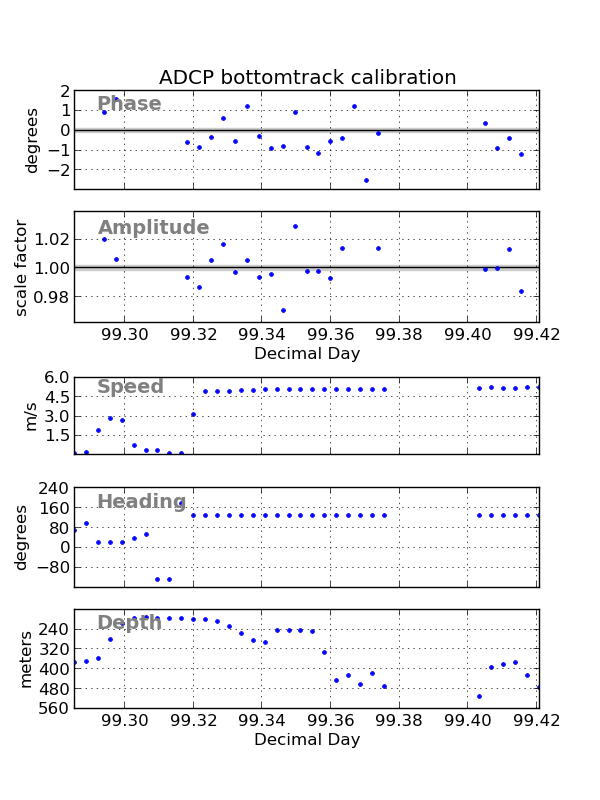
The results of an earlier calculation, with step size 1,2,3, is summarized below:
bottom track comparison
------------------------
step size 1 step size 2 step size 3
mean(std)
amplitude 1.0022(0.0138) 1.0019(0.0089) 1.0013(0.0088)
phase 1.8203(0.7633) 1.7374(0.4999) 1.7959(0.2805)
#pts used 16/24 14/23 13/22
out of total
We see the standard deviation decreasing as we increase the averaging, but also note that the values are very consistent. With step size 3, only every third estimate is independent, so the SEM is approximately 0.28/sqrt(13/3) = 0.13, versus SEM of 0.76/sqrt(16) = 0.19 for step size 1.
When finished, change back to processing directory:
cd ../..
2.8.11.5.2. 5.2 WATER TRACK CALIBRATION
This is part of quick_adcp.py calibration steps.
Return to TOP
Work is done in the cal/watertrk/ directory:
cd cal/watertrk
By default, quick_adcp.py uses the ship’s positions and the result of
adcpsect as_nav.tmp from the navigation steps (to provide
ship’s velocity relative to the reference layer). See this Python example for watertrack calculations.
The next step uses both these files to identify and calculate calibration parameters for each ship acceleration and turn. An acceleration or turn is detected based on the thresholds set in the control file:
pico timslip.cnt
The n_refs= parameter establishes a window of ensembles that bracket the jump or turn. We generally run this step using different window sizes to get a better picture, and then check for consistency across the results. For 5-minute ensembles, we normally set each run to:
settings
--------
nrefs= 5 7 9
i_ref_l0= 1 1 1
i_ref_l1= 1 2 3
i_ref_r0= 4 5 6
i_ref_r1= 4 6 8
always leaving out the 2 ensembles in the middle. The 5-reference window generally finds more points but also includes more noise. As the window gets bigger, fewer points become available but the averaging also tends to produce better results. Again, when we have both precision GPS and heading correction data, the 5 ensemble window usually gives the best results. Here we will look at all 3 window lengths.
The parameter use_shifted_times is set to 'no', meaning don’t apply any time correction when calculating amplitude and phase (the original purpose of timslip was to determine the time correction needed for the ADCP ensembles). We presume that we have done an adequate job of time correction during loading, unless timslip convinces us otherwise. If the ADCP times have been sufficiently corrected, then ‘nav - pc’ is normally under 5 seconds. If it becomes evident that there is some timing error, it is best to go back to the loadping stage and fix the times there.
timslip timslip.cnt
An example from a previous calculation shows the results of using
steps 5,7,9 for timslip in the watertrack calibration calculations.
Now we compare the results recorded in adcpcal.out.
Results:
-------------
nrefs 5 7 9
mean(std)
amplitude 1.01(0.0184) 0.99(0.0147) 1.00(0.0092)
phase 2.05(1.1302) 1.92(0.8186) 1.87(0.7607)
#pts used 15/19 16/17 13/17
over total#
The amplitude varies from 0.9959 to 1.0006, with lowest standard deviation (0.0092) for 1.00 (n_refs= 9). The phase varies from 1.87 to 2.05, with lowest standard deviation (0.7607) for 1.87 (n_refs= 9).
Looking at both bottom and water track results, we would normally pick 1.8 degrees as the angle, as this is roughly between the bottom track result for step=3: 1.79 and water track result for nrefs=9 of 1.87, which have the lowest standard deviation. We usually do not specify the angle to an precision beyond a tenth of a degree. The amplitude correction would be 1.00 (that is, none, usually specified to the hundredths place). With good data sets, especially those with gps heading correction data, we use higher precision: 0.01 degree in phase and 0.001 in amplitude. If we have, say, 200 watertrack points and a phase angle of 0.5, SEM is 0.035; so we do have a hope of getting accuracy beyond 0.1 degrees and we specify one more place.
Fortunately, this is relatively consistent with the results derived when the entire cruise (48 days’ worth of data) was used. So even though our subset has severe limitations, this gives us confidence to proceed and apply the above corrections to the database. It is worth noting that it is reasonable to take into account a larger body of information when determining the calibration values, if it is available. Such information might include calibration values from previous cruises on the same ship AS LONG AS nothing has changed (ie, the transducer hasn’t been removed and replaced; GPS heading antenna array has not been moved). We have found it helpful to combine timslip output from multiple cruises and run the watertrack calculation on the combination.
Now, we will rotate the data with both the heading correction values and the transducer offset calibration values.
When finished, change back to processing directory:
cd ../..
2.8.11.5.3. 5.3 ROTATION
To apply the calibration (phase and scale factor) to the database,
use the rotate command. This can be done using
quick_adcp.py --steps2rerun rotate --rotate_angle xx.xx --rotate_amplitude yy.yy
or can be done manually. Work is done in the cal/rotate/ directory:
cd cal/rotate
Edit rotate.cnt:
pico rotate.cnt
Specify DB_NAME, LOG_FILE (a running record of rotations performed on the database), TIME_RANGE: (or DAY_RANGE: or BLOCK_RANGE: or BLOCK_PROFILE_RANGE:; doesn’t matter in our case, we are rotating 'ALL'). For the gyro correction, we use the time_angle_file: option, and the amplitude and phase options for the bottom/water track values.
rotate rotate.cnt
actually rotates and rescales the U and V velocity components, (both water track and bottom track as we specified), and adds the file angle parameter and the constant angle to the variables ANCILLARY_2.watrk_hd_misalign and botrk_hd_misalign, and multiplies ANCILLARY_2.*_scale_factor by the amplitude factor.
Running showdb confirms that the data processing mask has been set to indicate rotation (second bit from the right), and the ANCILLARY_2 variable displays the rotation values used.
showdb ../../adcpdb/aship
Use option 1 to check the data processing mask, and option 16, variable ID 38 to view the changes to the ANCILLARY_2 variable.
When finished, change back to processing directory:
cd ../..
2.8.11.6. 6 PART 3: EDITING
Return to TOP
Editing involves making a few routine checks through the data, plotting the data to determine whether some correction is necessary, and applying the correction to the database as needed.
See gautoedit documentation for more details.
Threshold editing and manual editing write the flags to disk in files
with names like abadbin_tmp.asc, abadprf_tmp.asc,
abottom_tmp.asc, hspan_badprf.asc.
More information about PROFILE_FLAGS can be found here.
The following example applies flags from bad bin editing (flags in
a file called badbin.asc) to the database:
badbin ../adcpdb/aship badbin.asc
This simply sets the PROFILE_FLAGS variable in the database to indicate that particular bins have been tagged as bad. The original velocity values remain intact. During later access with ‘adcpsect’ or ‘profstat’, the user can specify whether to consider these tags during access by using the FLAG_MASK option. By default, this option is set to ALL_BITS, meaning data for bins at which PROFILE_FLAGS are nonzero will not be used. Use showdb, option 16 (GET DATA), variable ID 34 (PROFILE_FLAGS), to see the effects of running badbin on the database.
The following example applies flags from bad profile editing (flags in
a file called badprf.asc) to the database:
dbupdate ../adcpdb/aship badprf.asc
The file badprf.asc is created when entire profiles are flagged or marked bad. This sets the ACCESS_VARIABLES.last_good_bin to -1 to indicate that the entire profile is not to be used during subsequent access.
The following example applies flags from bottom editing (flags in
a file called bottom.asc) to the database:
dbupdate ../adcpdb/aship bottom.asc
This sets the database variable ANCILLARY_2.max_amp_bin to the bin indicated in the file, last_good_bin. It sets data processing mask bit 8 (bottom_sought), and clears bit 9 (bottom_max_good_bin), which allows further editing to be applied to the profiles.
Note that it does NOT set ACCESS_VARIABLES.last_good_bin, which access programs like adcpsect use during retrieval to determine the “good” portion of a profile (in addition to other editing criteria, of course, like percent good). The next program accomplishes this:
set_lgb ../adcpdb/aship
Again, use showdb option 16, variable ID 38 and 39 to see the effect of set_lgb on the database. The program updates ANCILLARY_2.last_good_bin, ACCESS_VARIABLES.last_good_bin to 85% of the minimum of the max_amp_bin from the bottom flagged profile and the two adjacent ones, as seen with BOTM_EDIT flag above, and the data processing mask (see the file eedit_chgs in codas3/adcp/doc for more detail). This is done only for profiles where the ACCESS_VARIABLE last_good_bin is not set to -1 (ie, those not flagged using badprf.asc).
Finally, edit setflags.cnt to set the PERCENT_GOOD threshold and add the option set_range_bit. This will set bits in PROFILE_FLAGS everywhere that percent_good falls below the minimum given or the bin falls outside the range in ACCESS_VARIALBES: first_good_bin to last_good_bin.
pico setflags.cnt
Now run setflags:
setflags setflags.cnt
If you care to check all the effects of this editing at this point, you can run through the stagger plots one more time, this time setting all flagging criteria in setup.m to []. Set PLOTBAD = 0 and EDIT_MODE = 0. Just plot ‘uv’ from beginning to end to check that you haven’t missed anything.
Other useful commands for use in editing include delblk and set_top. See descriptions in the Appendix.
When finished, change back to processing directory:
cd ..
2.8.11.7. 7 PART 4: DATA EXTRACTION
These steps are run with:
quick_adcp.py --steps2rerun matfiles
Return to TOP
2.8.11.7.1. 7.1 (part 1) time ranges
The tradional way to extract data from the database for
contouring (higher resolution) and vector plots (more averaging) is by
using adcpsect. . Since the primary key in
the database is profile time, we usually start by creating a grid
of time ranges. This may either represent some longitude/latitude
interval, or simply a time interval.
There are two ways to create the file with time ranges: llgrid and timegrid. The program llgrid converts a user-defined longitude and/or latitude grid to time ranges; the timegrid program simply creates a fiel with appropriately-formatted time ranges.
Example:
cd ../grid
pico llgrid.cnt
The lon_increment is set to some decimal degree interval (or a very large value to grid purely on latitude). The same is true for lat_increment. The lon_origin and lat_origin are usually set to -0.5 of the increment value to center the data on the grid boundary.
llgrid llgrid.cnt
creates an ASCII file of time ranges, which can be appended to the adcpsect.cnt file used to retrieve the data for plotting from the database. Review this file to see if the lon-lat increments are adequate to generate an acceptable averaging interval (the comments indicate how many minutes fall into each time range); normally, we want at least 2 ensembles for each average, but not too many either. It may sometimes be necessary/desirable to manually edit some of the time ranges to suit the purpose at hand.
The other program, timegrid, simply breaks up a time range into even time intervals.
NOTE: Do NOT use the “all” time option in timegrid.cnt; “all” uses default
beginning and ending times which cover a 100 year period. Timegrid does
not look at the database, but calculates even time intervals within the
time range(s) specified. If you want “all profiles”, use the “single”
option within adcpsect, or use the getmat program.
Example:
pico timegrid.cnt
timegrid timegrid.cnt
Again, the output file is meant for appending to adcpsect.cnt for extracting time-based averages.
When finished, change back to processing directory:
cd ..
2.8.11.7.2. 7.2 (part 2): Data Extraction
For coarser resolution (more averaging) we use the vector directory.
Example:
% cd ../vector
add timeranges with the include file option < @../grid/aship.llg > or
cat ../grid/aship.llg >> adcpsect.cnt
pico adcpsect.cnt
adcpsect adcpsect.cnt
This creates a *.vec file, which can be used as input to the vector
plotting program. The .vec file has columns lon, lat, (U, V) for
the first depth layer, (U, V) for the second depth layer, etc. in m/s.
The quick_adcp.py defaults for adcpsect only output *.mat files
For higher resolution we use the contour directory.
Example:
cd ../contour
add timeranges with the include file option < @../grid/aship.tmg > or
cat ../grid/aship.tmg >> adcpsect.cnt
pico adcpsect.cnt
adcpsect adcpsect.cnt
The quick_adcp.py defaults for adcpsect only output *.mat files
When finished, change back to processing directory:
cd ..
2.8.11.8. 8 DOCUMENTATION YOUR PROCESSING
Return to TOP
One of the most important steps in ADCP processing is documenting what has been done to the data. Ideally we would leave an accurate and concise record of all things of note and all the steps that were performed, so that someone else could come along later and reproduce all the processing, knowing exactly how it was done.
Modern processing directories have a file called cruise_info.txt
with one possible format for keeping track of the details.
2.8.11.9. 9 APPENDIX
Return to TOP
2.8.11.9.1. 9.1 Appendix Contents
2.8.11.9.2. 9.2 DELBLK
The command delblk should be used ONLY when you want to permanently remove from the database a range of data. You may specify the range by blocks, block and profile range, or by time range.
delblk adcpdb/aship

#% DATABASE: adcpdb/aship successfully opened
#
# Enter one of the following numbers :
#
#  1.  Delete block(s)
#  2.  Delete block-profile range
#  3.  Delete time range
#  4.  Exit program
#
# ==>
#-----------
#Enter your choice; you will be queried from the range
#   specifcations, with a description of the format expected.
2.8.11.9.3. 9.3 MISCELLANEOUS COMMANDS
Return to TOP
lst_conf lst_conf.cnt
Extract the history of the configuration settings from a CODAS database into a text file.
lst_prof lst_prof.cnt
Produce a list of times and positions of selected profiles within the given time range(s) from a CODAS database.
mkblkdir mkblkdir.cnt
Generate a new CODAS database from a set of CODAS block files. The new database will consist of a new block directory file and a copy of each input block file, converted if necessary to the host machine format.
getnav getnav.cnt
Retrieve the navigation information for selected profiles within the given time range(s) from a CODAS ADCP database.
NOTE:
getnav gets positions from the NAVIGATION data structure where they are placed by the user exit program. UH user exits place an end_of_ensemble fix; RDI’s NAVSOFT places an ensemble-averaged fix. The NAVIGATION data structure is not updated by any CODAS processing steps.
lst_hdg lst_hdg.cnt
Extract the ship’s mean heading and last heading from a CODAS database into a text file.
nmea_gps nmea_gps.cnt
Convert NMEA-formatted GPS fix files to a columnar text format suitable for use with the codas3/adcp/nav programs, and/or to Mat-file format for Matlab.