2.8.1. Tool: patch_hcorr.py
This tool is used to filter or edit the time-dependent heading
correction. At it’s simplest, it interpolates through gaps in the
heading correction – in many cases this is sufficient. The program
patch_hcorr.py reads the file cal/rotate/ens_hcorr.asc and
plots useful variables in a graphical interface that gives access to
filtering options and manual editing.
2.8.1.1. When should we use this tool?
For example:
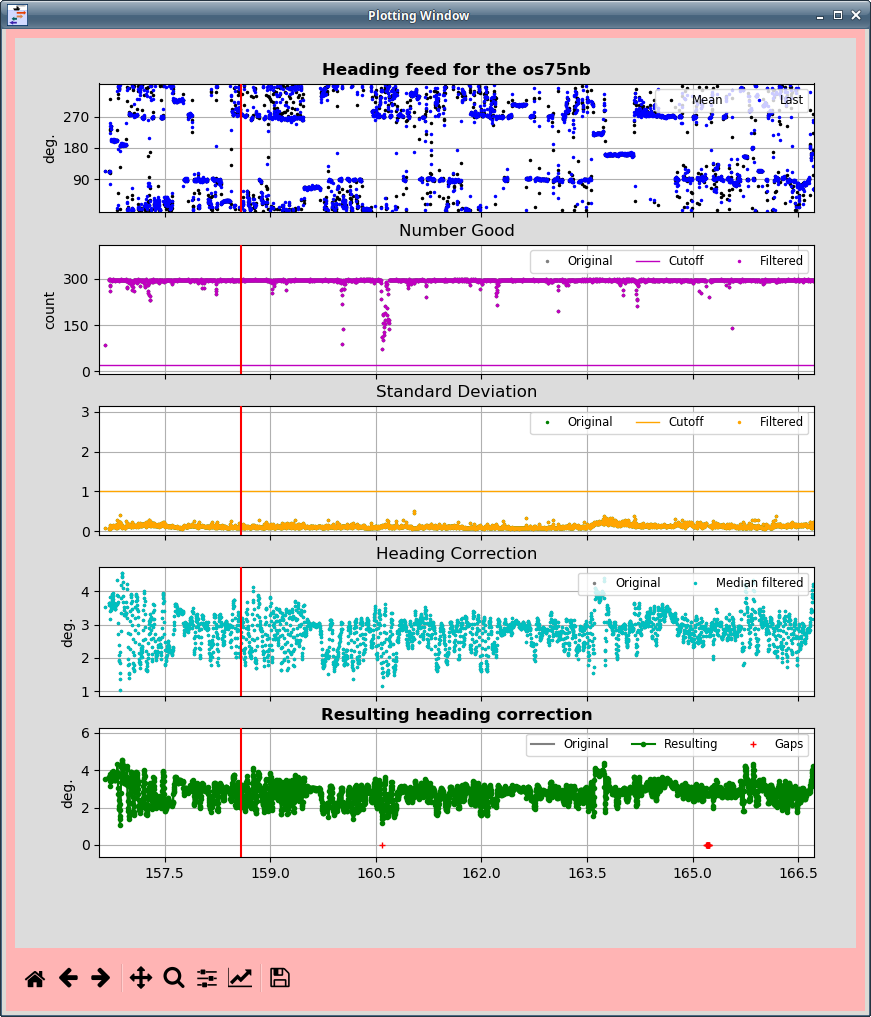
First, inspect the heading correction figures in cal/rotate/ens_hcorr*.png:
figview.py cal/rotate/*.png
Look for gaps (red crosses ‘+’ on the graphic)

The green dots indicate the correction from the gyro (reliable heading device) to the accurate heading device (Ashtech, in this case) for each of the 5-minute profiles. There is one gap in the heading correction that starts on the decimal day 165.2 and on the bottom of this figure it is possible to see the red crosses ‘+’ (just above the 165.2). The heading correction is around 3deg, but when the ashtech failed briefly the missing values were filled with a zero (red crosses ‘+’ on the graphic).
Because the data are generated near-real-time, we cannot interpolate
during data acquisition, but in postprocessing we can, because we know what
the value of the correction is after the ashtech returns. We can write code
to interpolate through that gap, or we can use patch_hcorr.py.
Because the heading correction was quite stable just before and after the gap, a linear (straight line) interpolation from the last available data (green dot) to the first one after the gap, should be a reasonable estimate.
Second, Look at the velocities directly using:
dataviewer.py
The top half of this figures has panels:
top panel: ocean velocity u (east/west)
middle panel: ocean velocity v (north/south)
lower panel: green = ship speed, pink = ship heading
The bottom half of the figure shows the cruise track with the velocity as vectors.
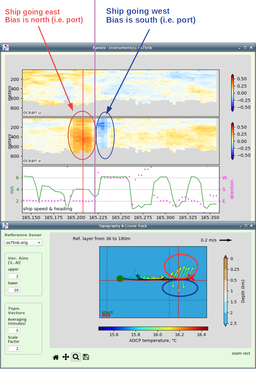
The ship was heading east at the beginning of the gap, and west at the end of the gap (pink dots in the bottom panel).
Heading errors result in ocean velocity errors that are to port or starboard, i.e. athwartship, not in the direction the ship is going. It is consistent that the ship was going east and then west, and the velocity error is entirely in the north and then south direction, in this case always to the left of the ship.
The vertical red line in the top plot is at the location of the red crosshair in the vector plot.
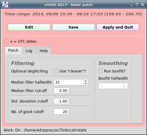
Now run patch_hcorr.py:
cd  cal/rotate
patch_hcorr.py
Note
This program has three sections:
Editing and filtering
Save and preview results
Apply and Quit
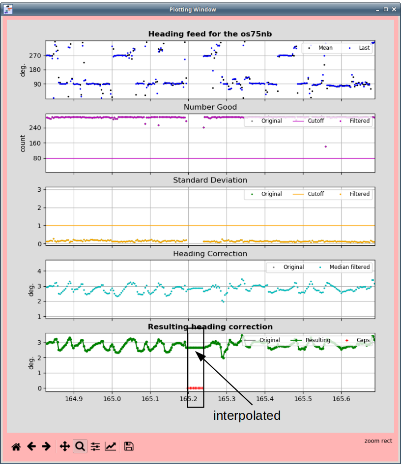
(1) Editing and Filtering
Two windows will pop up:
The plotting panel showsplots of the heading correction for each of the 5-min ensembles in the dataset.
The panels are:
mean and last heading in the ensembles.
the number of good points in the heading correction estimate
standard deviation of the estimate
heading coorection and the median filtered version (not relevant when you start)
original and final estimate, and gaps (in red)
The control panel has various functionality for filtering and editing, but the primary use is to view and interpolate. This section will be expanded (at some later date) to illustrate them:
deglitching (a second-derivative filter)
median filter
standard deviation cutoff
number of good points
run a box filter on the final results
There is also a manual editing scheme that is similar to the edit mode of dataviewer.py (see this link for further details)
If we zoom in on the bad section we can see the red ‘+’ signs where the data were bad (last panel, decimal day 165.2) and above it, the green heading correction values, including the interpolated part.
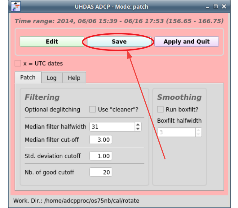
(2) Save and preview results
To write the new heading correction data to the disk, click on the “Save” button:
A window pops up with a preview of the original heading corrections and the new heading corrections. Check that things look good (did the correction do the right thing?)
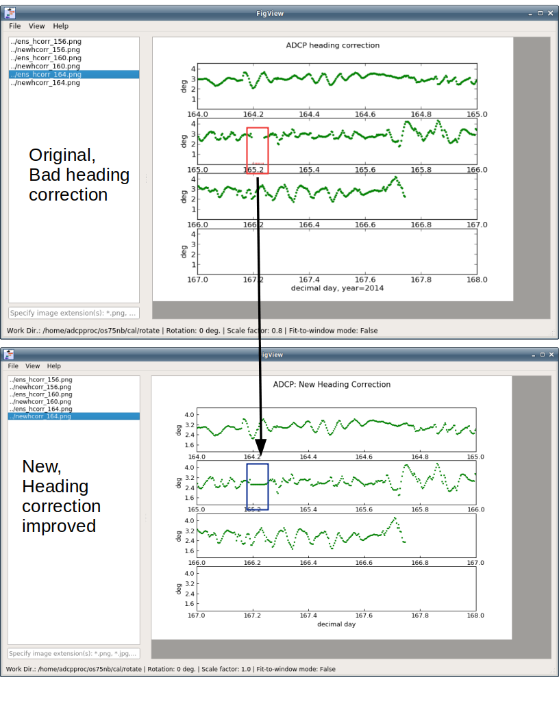
If you don’t like the results, continue to change filtering and editing, try “save” and review.
When you are satisfied, click Apply and Quit
Note: Make sure to close the figview window beforehand otherwise the “Apply and Quit” button will stay disabled.
(3) Apply and Quit
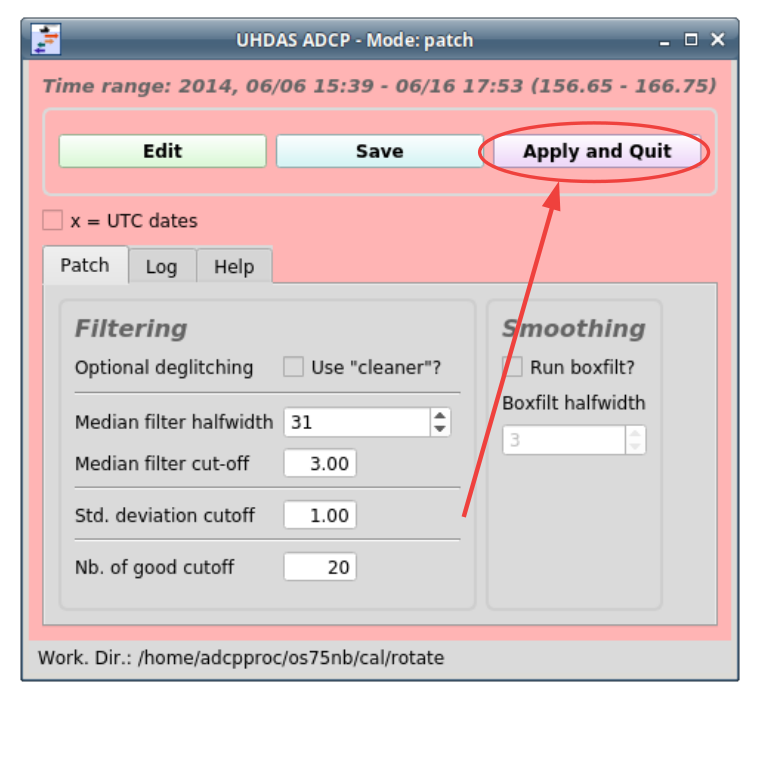
A warning pops up to verify that you want to take the next steps.
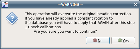
If you click ‘yes’ it will run these commands (from the cal/rotate directory,
where you ran patch_hcorr.py):
rotate unrotate.tmp
rotate rotate_fixed.tmp
cd ..
quick_adcp.py --steps2rerun navsteps:calib --auto
A window pops up showing the original and new watertrack calibrations:

And a text message is printed to the command-line terminal where you ran the program. It will say something like:
The following commands were run:
-------------------------------
cd /home/adcpproc/project/os75nb/cal/rotate ; rotate unrotate.tmp
cd /home/adcpproc/project/os75nb/cal/rotate ; rotate rotate_fixed.tmp
cd /home/adcpproc/project/os75nb ; quick_adcp.py --steps2rerun navsteps:calib --auto

---Original Calibration---
- Water Track Calibration:
            median     mean      std
amplitude   1.0050   1.0052   0.0100
phase      -0.0640  -0.0480   0.5879


---New Calibration---
- Water Track Calibration:
            median     mean      std
amplitude   1.0060   1.0060   0.0087
phase      -0.0870  -0.0531   0.4793


You can now apply the final calibration by running:
    quick_adcp.py --steps2rerun rotate:apply_edit:navsteps:calib --rotate_amplitude AMP --rotate_angle PHASE  --auto
Where AMP and PHASE are the values indicated in the watertrack (or bottomtrack) calibration output.
See https://currents.soest.hawaii.edu/docs/adcp_doc/codas_doc/calibration/index.html
Warning
Note that the new (fixed) time-dependent heading correction has been applied but any constant rotation has been reset to 0, and any amplitude has been reset to 1. Be sure to check the calibration and see if you need to apply calibrations again.
Now compare the “original/backed-up” dataset against the “patched” one using dataviewer in compare mode and check again the profiles on the date when the gap happens:
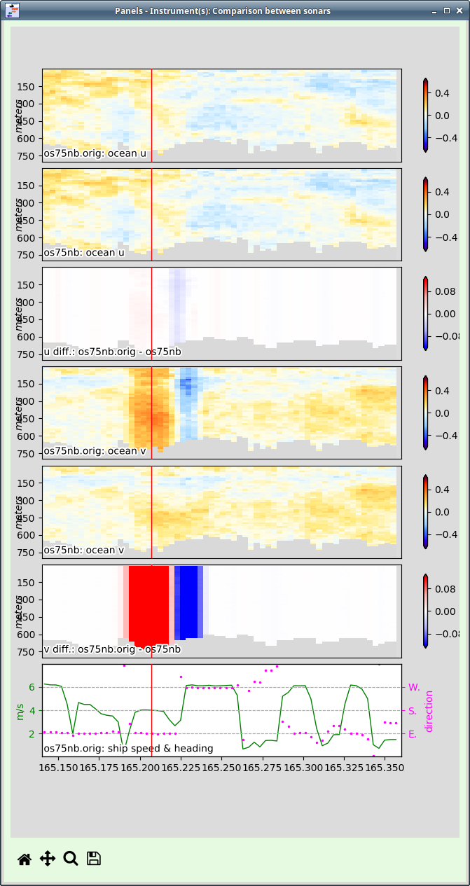
And it looks much better now!