. ……………………………….. .. UHDAS/CODAS restructured text document .. ………………………………..
2.6.2. Edit Mode
This is the fourth generation of graphical editing tools for CODAS data. In all cases, data are flagged as ‘bad’ based on one of three criteria:
bad (due to some threshold)
below the bottom
manually excluded
Once the ‘bad data’ are flagged in the graphical editor, a separate step to “apply editing” to the CODAS database involves writing the flags to ascii files and applying the information in those ascii files to the CODAS database so that further data extraction will not show those flagged values.
This html documentation is meant to give you an introduction to the
dataviewer.py and provide some guidance as to its use. Figures
may not look exactly as they do on your computer: some
screenshots are taken under Mac OSX or Linux interfaces, and some
figures illustrating editing concepts are retained from the earlier
Matlab gautoedit tutorial. This is a work in progress; some of
the screenshots are still from the python2 version.
2.6.2.1. Overview of the Windows
The original editing tool was written in Matlab. The original Python version only works in Python2.7, because of the graphical library used (Wx). This version works with Python 3.6 using the Qt graphical library. It is more sophisticated than the Wx version, but retains the same strategy as its ancestors.
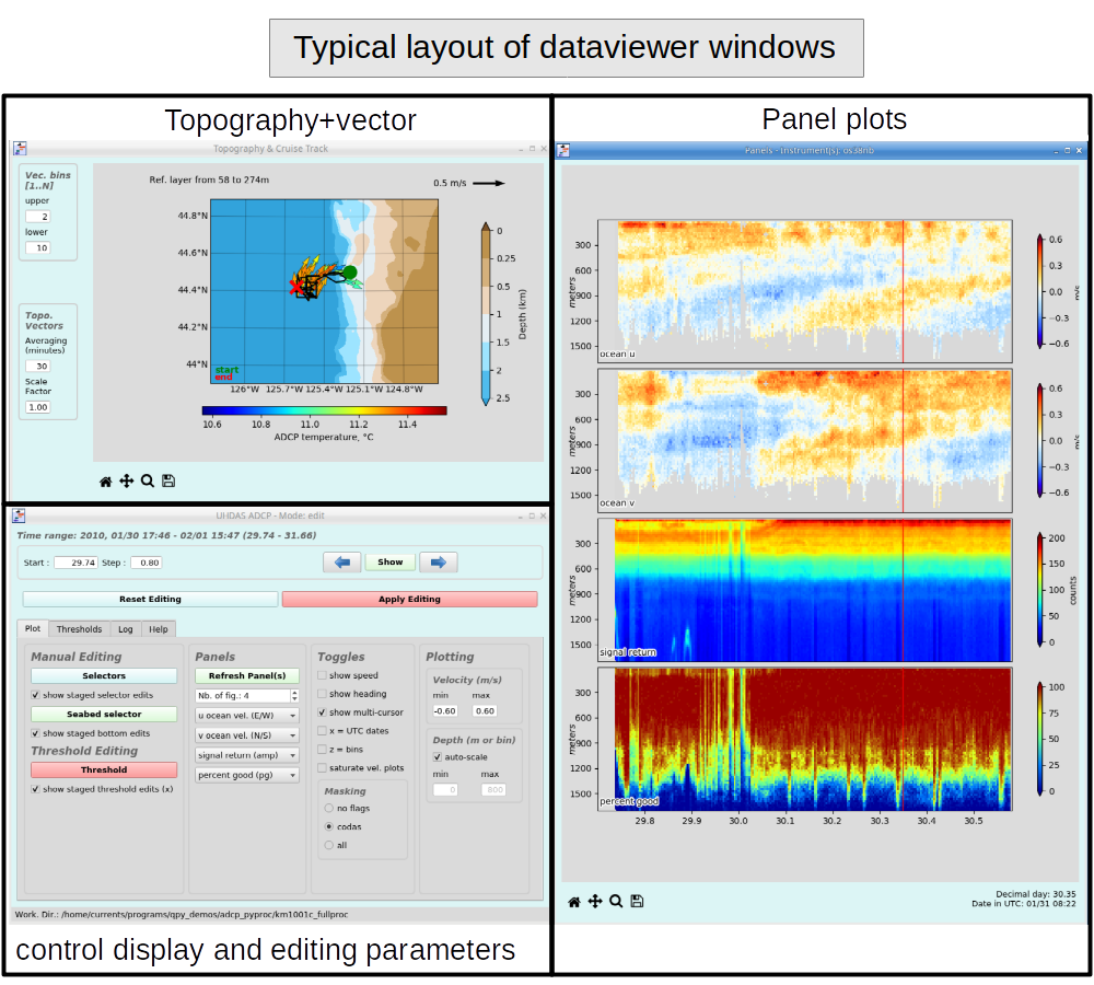
CONTROL PANEL: display and editing parameters are controlled here |
|
PANEL PLOT (typically u,v, percent good, amp) |
|
VECTOR PLOT of surface velocity over topography |
|
The work flow below assumes each sonar processing directory has already had:
heading correction patched (if required using patch_hcorr.py)
calibration (phase and possibly amplitude using quick_adcp.py) applied
transducer-ADCP offsets applied (using quick_adcp.py)
Overview of editing work flow:
For each sonar (eg. wh300 and os75nb):
Edit a chunk of data, click Apply Edits, go to the next time range.
Editing uses these two schemes:
manual selection (Plot Tab)
threshold editing (Threshold Tab)
Repeat for subsequent time ranges, working through the whole cruise
After going through the cruise
review the data from the whole cruise again.
repeat as needed.
After editing, adjust the phase amplitude calibrations again so they are as good as possible
Then step back and use compare mode to flag more data if that is necessary
2.6.2.2. More Details about each window
When dataviewer.py -e is invoked, three windows appear.
Here is an example of the window layout for editing
(click thumbnail for a larger image):
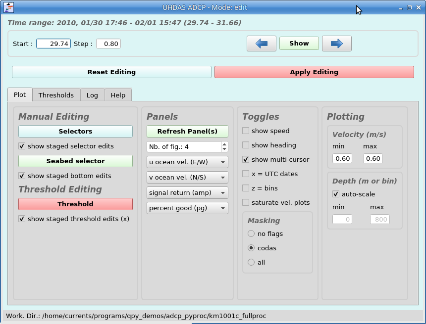
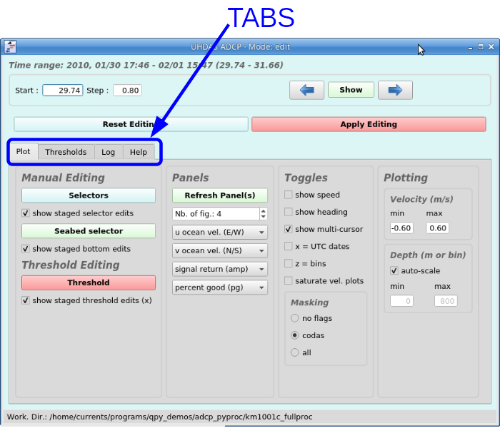
Control Window:
- The Dataviewer Edit Mode has 4 tabs.
Plot: (control what is viewed)
Thresholds: control threshold editing (see below)
Log: show time ranges requested so far
Help: a little help (under construction). Most help is in the web pages you are reading right now
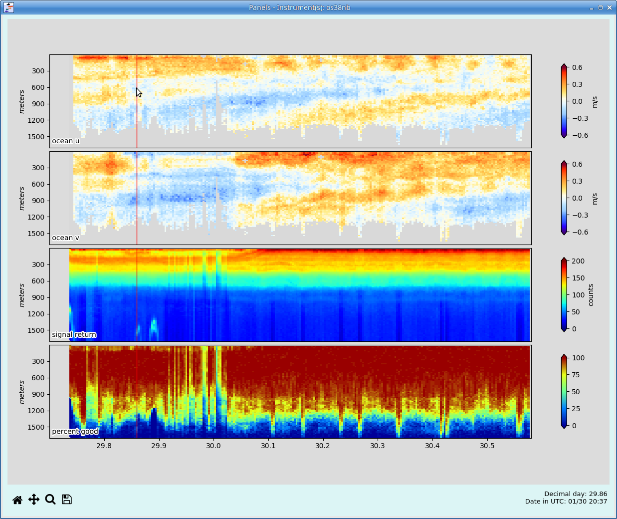
Panel Window:
The only thing you can do in the panel window is pan or zoom, but if Multicursor is enabled in the Control window, the red line in the panel plot matches the corresponding position in the topography window.
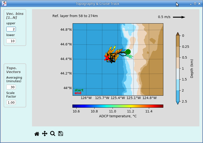
Topography Window:
The topgraphy window is designed to view ocean velocity vectors over ocean topgraphy. You can change some of the display settings (vector averaging in vertical and time, and length of vectors). You can pan and zoom (but the topography does not increase in resolution). If Multicursor is enabled in the Control window, the red line in the panel plot matches the corresponding position in the topography window.
2.6.2.3. Work Flow (Editing ADCP data)
2.6.2.3.1. Starting out
Run
dataviewer.py -efrom your ADCP processing directory or theeditsubdirectory.
dataviewer.py -e
Choose the number of days to display (based on your screen resolution), make sure you can see individual profiles.
Press “Show” to load the data from that time range
Typical Editing Steps
Note
Note that the following are often equivalent:
clicking Show
after entering text, hitting the Return key
ACTION TO TAKE |
WHAT IT DOES |
|---|---|
|
Shows the chosen time range with thresholds updated |
|
You can enable/disable threshold editing, and you can adjust values |
|
|
|
Thresholds: enable, then tweak Seabed Selector: click on the bin with hightest amplitude; doubleclick to stop. Sidelobe effects ARE accounted for. |
|
|
|
Applies thresholds and manual editing for present time range |
|
Resets flags for selected profiles to minimum Percent Good only (in database); Shows effect of thresholds in the view |
|
Assume this will take two passes. Flag obviously bad values; do not yet flag subtle problems. Investigate later |
|
Move forward in time by “step” (with a slight overlap |
NOTES
When Apply Editing is clicked:
flags from files ending in
*.ascare applied to the database.flags from all
*.asc filesare then appended to*.asclogall
*.ascfiles are deletedThe
*.ascfiles with flagging information can come from
earlier editing session (automatic editing during at-sea processing, older editing session)
the present state of threshold settings
2.6.2.3.2. Manual Editing Examples
Look at the data with different masking (select different collections of editing flags to display) This example is a newly-loaded LTA dataset; no editing has occurred except for a percent-good cutoff of 50% (PG)
diagnostic: no flags (shows everything in the database)
default: codas (shows data in CODAS database that is not flagged)
diagnostic: all flags are applied, CODAS flags and threshold flags. This helps visualize what your dataset will look like if you click “Apply Editing”.
Adjust threshold editing if necessary (see below); click “Show” to renew the plot
You might have velocities below the bottom.
First see how much the Threshold editing can remove
Try turning on Bottom Identification
Try adjusting the bottom-detection parameter.
Or you can use the Seabed Selector to manually identify the bottom:
Manually edit out the bad data associated with the bottom.
The bottom editing tool always uses “amp” for editing
The bottom edit tool takes the beam angle into account (side-lobe interference) so all you should have to do is choose the maximum amplitude (or a bin above that).
Editing by bins or profiles using Selectors
Note
Select a bin or profile by grabbing the middle, not a corner.
The Selectors window has
dropdown menu for variables plotted, including ocean u, v, percent good, signal return, and others.
dropdown menu for editing tools:
Rectangle: click and drag to select the rectangle of bad bins – the rectangle will be selected when the mouse button is released.
Horizontal Span: click and drag the mouse horizontally to select profiles
Vertical Span: click and drag the mouse vertically to remove all the bins in a specific range
One click: click in a bin
Polygon: Use single clicks to create a polygon. To finish, go back to the first point and click (it will “grab” that point if you get close enough)
lasso: freehand draw. Lift the mouse button to release, and it will connect to the beginning of the curve.
Note
In the Selector window
you can add edits using any of the tools or variables.
use Mask mode to ADD flags
use Unmask mode to SUBTRACT flags
If you don’t like any of your editing you can
close the manual editing window without doing the Stage Editing step
click “Clear Edits” to reset to its initial values
the flags are not applied to the database until you click “Apply Editing” in the Control Windwow.
Note
After “Apply Editing” you can revert to just minimum Percent Good by using the button to Reset Editing (selected profiles are reverted). More detail here
Note
Sometimes you need to reset editing manually. Instructions for that are in this link
2.6.2.3.3. Threshold editing
Wire interference and ringing
wire interference
set the number of bins to evaluate
set the ship speed (only looks when ship is slower)
enable/disable: set Error Velocity cutoff (best signature for wire interference) – this value is smaller than the general error velocity criterion below
This algorithm finds bad bins, and then also flags each bin to the right and left, and above and below. It is designed to hollow out a little patch around a peak of high EV. It is not simply a threshold.
ringing
set the ship speed (only looks when ship is faster)
enable/disable: set number of bins to reject
Thresholds for excluding individual bins
These are all disabled be default. None of them is good enough to really do the job, but they can be used together or as indicators of a problem
error velocity: (good indicator of a problem)
vertical velocity: (specialty: sometimes useful for bizarre cases of electrical interference)
shallow low Percent Good: (can be useful for cases of ringing, bubbles, or ice). It cannot get rid of everything but is sometimes a good indicator (example)
resid_stats_fwd: a measure of how consistent the averages are in the direction of ship’s travel. This is a diagnostic for intermittent underway bias at the single-ping level.
Percent Good in Reference Layer
This is a way to require a minimum number of high Percent Good bins in a reference layer in order to accept the profile. It can be useful in situations with intermittant bad weather and periods with few, isolated profiles
choose the range of bins to asses
choose the Percent Good cutoff for bins in that reference layer
choose how many good bins are required for a profile to “pass”
Identify Bottom
Try turning on Bottom Identification
Try adjusting the bottom-detection parameter.
Thresholds for excluding whole profiles
jitter: obsolete: a somewhat arbitrary indicator of “data smoothness” (was more important in Matlab processing; Python processing is better and produces less “jittery” data
neighbors: if profiles are are gappy, but profiles adjacent to the gaps seem bad, this will trim them
ship speed: discard if ship speed exceeds this; useful if the heading device has poor accuracy
2.6.2.3.4. Interpretation: things to keep in mind
2.6.2.4. Finishing up
After you have reached a stopping point, eg. “the whole dataset”, run this command to ensure a clean sweep of any remaining ascii files, rerunning the navigation steps and updating calibration: (This is done from the processing directory)
Now look at the dataset again using dataviewer.py to be sure you
edited out all the bad parts. There’s often something left,
so it’s worth checking.
(Return to TOP)