2.2. Demos: Overview and Directory Layout

2.2.1. Overview

The first tutorial demonstrates typical steps post-processing steps for a UHDAS dataset acquired at sea.

Note

You really need to do the postprocessing demo first. Then it’s relatively easy to go through the steps necessary for your scenario using adcp_database_maker.py. If for some reason that doesn’t work, the last set of demos shows you the actual steps going on behind the scenes, in case you need to do things more manually.

To create the directory used in post-processing two datasets are used: UHDAS and VmDAS. These will be demonstrated using adcp_database_maker.py. Additional demos will show how to obtain the same data results using command-line steps.

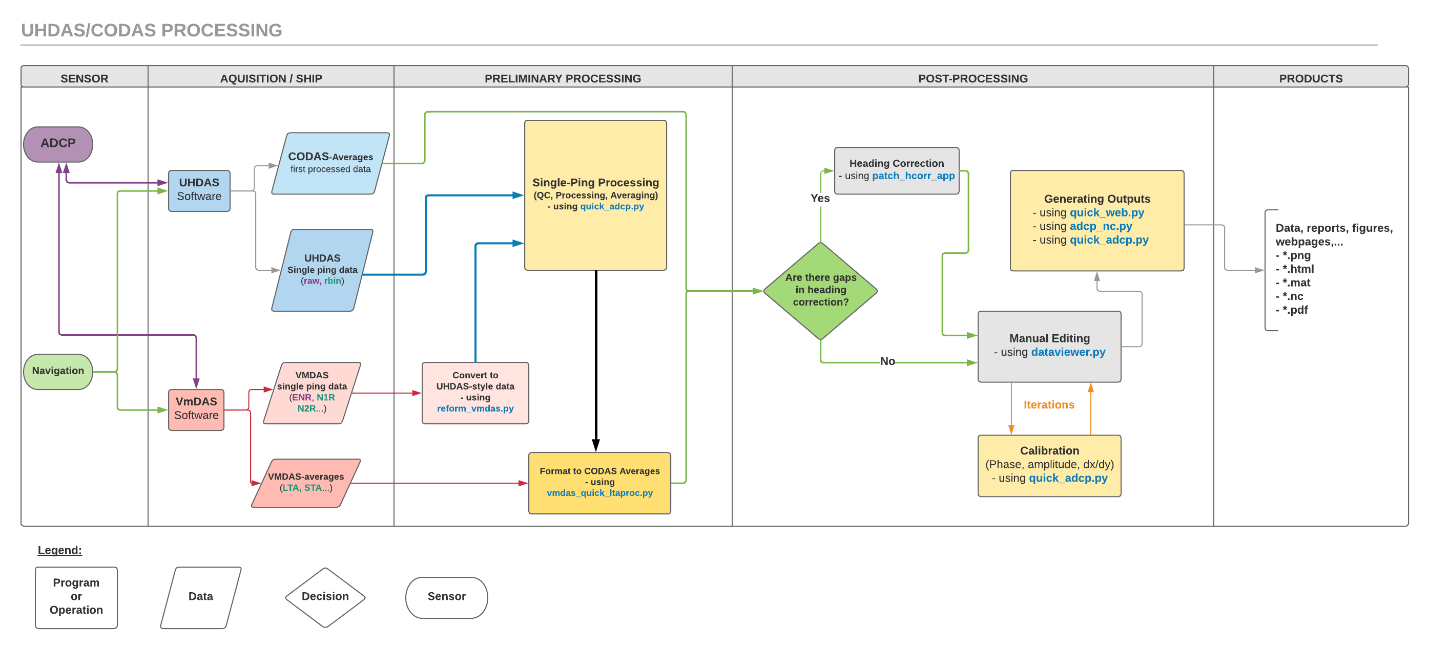
The examples that follow use two datasets for practice, one is UHDAS Data and one is VmDAS Data. UHDAS data includes two flavors: the entire raw single-ping data, stored in a directory structure with specific file names; and the pre-processed data from the at-sea UHDAS processing. which contains ocean velocities in earth coordinates. VmDAS also has single-ping data (ENR,N1R,N2R files) and averaged data in earth-coordinates (LTA or STA).

The processing examples that follow use the data from the adcp_py3demos*.zip files mentioned in the CODAS Installation instructions. Paths given below match the virtual computer, for simplicity. For example, on the virtual machine:

• the adcp_py3demos source is in: ~/adcpcode/programs/adcp_py3demos

• the examples use ~/my_adcp_py3demos to do the demos.

Instructions for each processing example exist in four places:

• using adcp_database_maker.py: these adcp_py3demos tutorials

• basic instructions: quick_adcp.py command-line help

• annotated instructions: see links in each section

• with metadata: the text files associated with the processing (in the adcp_py3demos/adcp_pyproc directories) have the same (basic) instructions, with additional meta-data included. These completed files are a good example of what to submit with your data when you send it in to the Joint Archive for Shipboard ADCP, JASADCP

Note

You should work through the post-processing demo because no matter what kind of data you have (VmDAS or UHDAS) ultimately you will need to know how to do the post-processing.

The demos cover these scenarios:

POSTPROCESSING

1. postprocessing a dataset collected by UHDAS at sea

2. VmDAS post-processing demo (referred to in VmDAS LTA demos below)

PRELIMINARY PROCESSING

3. adcp_database_maker.py

   1. UHDAS data

   2. VmDAS LTA (or STA) data

   3. VmDAS ENR (single-ping) processing

4. commandline demos

   1. UHDAS data using command-line steps

   2. “vmdas_quick_ltaproc.py” command-line

   3. LTA data using command-line steps

   4. ENR data using command-line steps

There is also a rudimentary “PINGDATA” demo, using the original 1993 pingdata. The “original pingdata demo” has a very detailed manual, but the manual was written for Matlab processing (so some parts are different). The new Python pingdata demo exists in the text+directory form (no html documentation) alongside the other demos, and in quick_adcp.py --help. There is not a web page for the pingdata demo.

The glossary describes some of the terminology.

This figure describes the demo directory structure and how it ties to the terminology.

This ascii file shows the layout of the demo directory in more detail.

(Return to TOP)

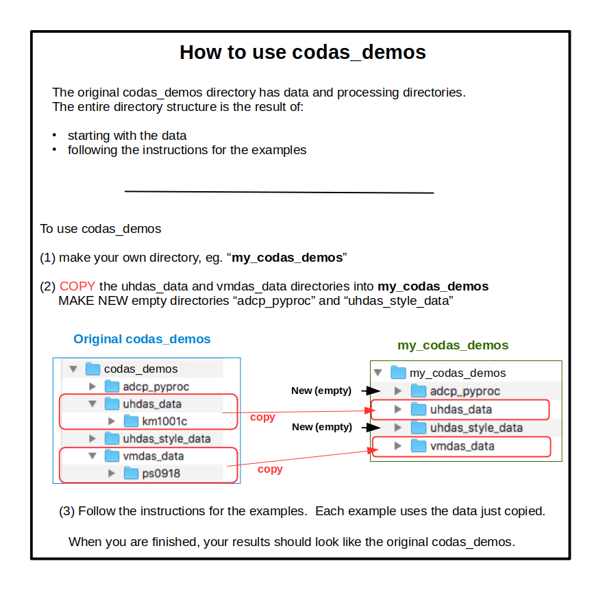
2.2.2. Demos: Directory Setup

The adcp_py3demos directory is both an example (of what a final data processing directory looks like) and the source (of the data for these examples). If you start with the directory structure described below, your final processing directory should be nearly identical to adcp_py3demos/adcp_pyproc.

Before you start working with any of the demos, make your own directory to store the data and practice processing. The examples assume you have already set up a working directory such as below. The command-line examples are designed to copy-paste and use in the virtual computer. A graphical example is shown below.

Check out the glossary for these terms, used below:

• Project Directory

• Processing Directory

• UHDAS Data

• VmDAS Data

• UHDAS-style Data

---

1. make a directory called my_adcp_py3demos to hold your practice demos

   example:

cd
ls
mkdir my_adcp_py3demos
cd my_adcp_py3demos
pwd

---

The result should be:

/home/adcpproc/my_adcp_py3demos

2. Copy the uhdas_data directory from the example into my_adcp_py3demos, just as you would if you were getting the data from an at-sea disk

   example:

cd ~/my_adcp_py3demos
cp -a  /home/adcpcode/programs/adcp_py3demos/uhdas_data  .
ls uhdas_data

The result should be:

km1001c

---

3. Copy the vmdas_data directory into my_adcp_py3demos

   example:

cd ~/my_adcp_py3demos
cp -a  /home/adcpcode/programs/adcp_py3demos/vmdas_data  .
ls vmdas_data

The result should be:

ps0918

---

4. Make a directory called uhdas_style_data (for converted VmDAS data)

   example:

cd ~/my_adcp_py3demos
mkdir uhdas_style_data
ls

The results should show 3 directories, all related to data:

uhdas_data  uhdas_style_data  vmdas_data

---

5. Make a directory called adcp_pyproc (for your UHDAS and VmDAS projects)

   example:

cd ~/my_adcp_py3demos
mkdir adcp_pyproc
cd  adcp_pyproc
pwd

The result should be:

/home/adcpproc/my_adcp_py3demos/adcp_pyproc

---

6. Make one project directory for each dataset. All your processing examples related to that dataset will be in the associated project directory.

   example:

cd ~/my_adcp_py3demos
cd  adcp_pyproc
pwd
mkdir km1001c_uhdas
mkdir ps0918_vmdas
ls

The result should show the two project directories:

km1001c_uhdas  ps0918_vmdas

---

These steps are summarized here (copy-paste text suitable for the CODAS virtual computer).

All the examples will refer to adcp_pyproc. You will be building up your own version, but the directory structure and files of a finished version exist in your data source for the demo. Click the image below to enlarge

(Return to TOP)

---