2.3. UHDAS Post-processing Demo
Scenario:
A disk exists with ADCP data collected at sea by UHDAS. Preliminary processing has already been done by the automated programs on the ship.
The processing directory is ready for the next steps
Everything seems to have worked; the data look good. All that remains is to edit out in-port data and a few bad profiles, and apply a small calibration correction.
Resources
command-line help:
quick_adcp.py --commands postproctext file (with metadata) from actual final processing directory
dataviewer.py documentation (viewing and editing)
the rest of this web page
Note
Directory Strategy
To simplify the documentation, these instructions assume you have set up your directories as in the Directory Setup section, and you are doing your processing demos in my_codas_demos/adcp_pyproc
your practice directory                        source
-----------------------                       -----------

my_codas_demos
my_codas_demos/adcp_pyproc                 (new, WORKING IN HERE)
my_codas_demos/uhdas_data                  copy of codas_demos/uhdas_data
my_codas_demos/vmdas_data                  copy of codas_demos/vmdas_data
my_codas_demos/uhdas_style_data            (new, empty, for VmDAS conversion)
Identify the CODAS Averages from the disk. These directories are usually located under the
CRUISE_NAME/proc/folder and are named after their associated sonar (e.g.km1001c/proc/os38nb).In your work area (
adcp_pyproc), make a Project Directory for all tutorials related to the cruise km1001c data.:cd ~/my_codas_demos/adcp_pyproc mkdir km1001c_uhdas cd km1001c_uhdas pwd
The result should be:
/home/adcpproc/my_codas_demos/adcp_pyproc/km1001c_uhdas
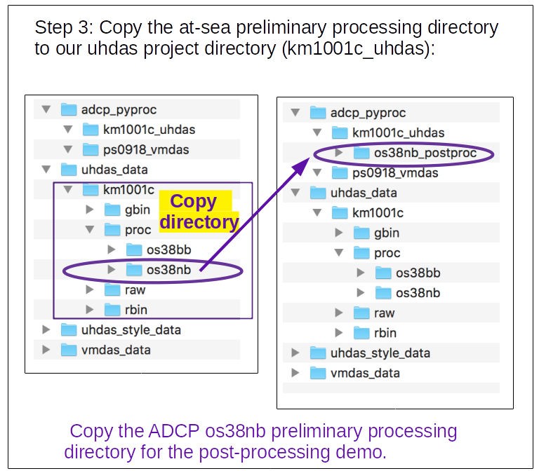
This the postprocessing demo, so we want to use the at-sea preliminary processed data from the cruise data. Copy the whole ADCP processing directory for this example (
os38nb) to your postprocessing locationCopy this directory:
~/my_codas_demos/uhdas_data/km1001c/proc/os38nb
to this location:
~/my_codas_demos/adcp_pyproc/km1001c_uhdas/os38nb_postproc
Note
We will use the cp (copy) command. If you want to see what is happening in your command, add the verbose option cp -av
From the project directory (km1001c_uhdas) run this:
cp -a ../../uhdas_data/km1001c/proc/os38nb os38nb_postproc
ls
The result should be:
os38nb_postproc
Now you should have:
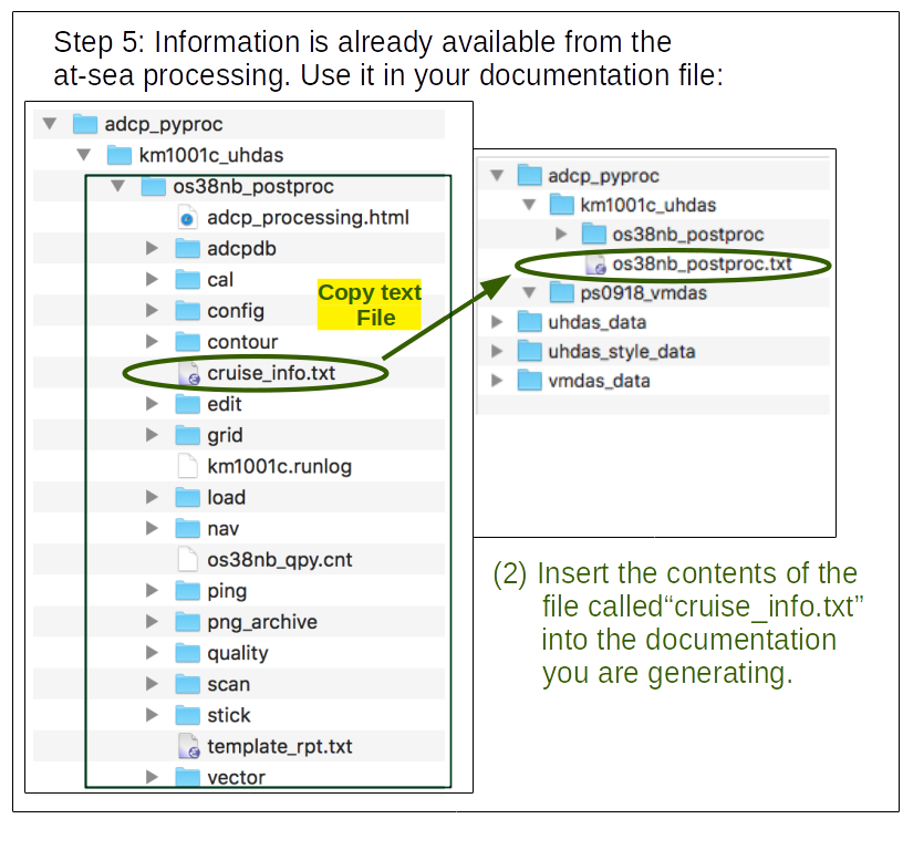
For each processing directory, keep notes in a text file (not a word-processor file) about your processing, eg.
os38nb_postproc.txt. This should be adjacent to the processing directory.We will pre-fill the text file with contents of the file
os38nb_postproc/cruise_info.txt. Valuable metadata reside in the cruise_info.txt file. It’s not complete, but it’s a start. From the project directorykm1001c_uhdas, type this:cp os38nb_postproc/cruise_info.txt os38nb_postproc.txt ls
The result should show:
os38nb_postproc os38nb_postproc.txt
Now you should have:
You can use a variety of editors, but one which we install
on all CODAS virtual machines is emacs. Emacs is a powerful
editor that includes a standard graphical interface. The & at the end
gives you the command-line prompt back.
emacs os38nb_postproc.txt &
Instructions
start making notes
Copy and paste this in your text file, at the end of the existing text:
Cruise km1001c processing:

The os38nb at-sea processing directory was copied from
the "proc" directory of the km1001c cruise disk.

All postprocessing is done with full codas+python (i.e. using
numpy+matplotlib)

(1) make a **project directory** ``km1001c_uhdas`` for work done
    related to this cruise

   - copy km1001c/os38nb directory from uhdas_data directory into km1001c_uhdas
   - rename it os38nb_postproc (to distinguish it from the other demos)
   - start editing a text file called os38nb_postproc.txt, with the
           contents of os38nb/cruise_info.txt at the top.
   - keep notes down below, and fill in above later
Look at the evidence in the processing directory to see if this is what we expect, look for problems, evaluate what needs to be done. Write this down: you want to be able to remember what you did. Your notes should be inside the project directory so if you need to delete the processing directory, you don’t lose your notes as well!
This is our goal for the final text file: (here)
Compatibility with older cruises
Because we are post-processing an older directory (Matlab processing), there is a file which contains crucial metadata, and it is missing.
This is the command we want to run, but it will fail because dbinfo.txt is missing:
quick_adcp.py --steps2rerun calib:navsteps --auto
If you are processing your own data, try that first. For this older
cruise we must generate the metadata file dbinfo.txt before we can
edit or correct calibrations, thus bringing the dataset into
compliance with modern tools.
Note
To bring this processing directory up to date, run the following command (this command should be run as ONE LINE)
quick_adcp.py --steps2rerun navsteps:calib --datatype uhdas --sonar os38nb --beamangle 30 --yearbase 2010 --ens_len 300 --cruisename km1001c --auto
This is the only time we need to run such a long command for this cruise. This link explains in more detail.
Remaking PNG Figures
It is also a good idea to remake the figures (to take advantage of improvements in the software):
quick_mplplots.py --yearbase 2010 --plots2run all --noshow
The last thing we will do is to make a COPY of the processing directory before we start changing things, so we can compare the effects of our work:
cp -a os38nb_postproc os38nb_postproc_orig
Note
Now we switch to working inside the processing directory.
All commands related to editing or calibration of the dataset
are run from the processing directory, os38nb_postproc
unless otherwise noted – go there now
cd os38nb_postproc
pwd
The result should be:
/home/adcpproc/my_codas_demos/adcp_pyproc/km1001c_uhdas/os38nb_postproc
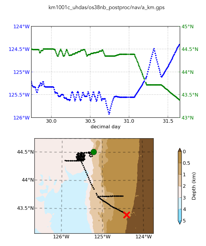
Look at the cruise track to see what we’re expecting:
plot_nav.py nav/a_km.gps
This is a cruise with a “patch test” to calibrate the multibeam. The ship started this “cruise” near the patch test site, did the patch test, then came down towards Newport, Oregon and did a reciprocal run in towards shore and back out, then proceeded to port.
There should be ample watertrack calibration points from the patch test.
Click on the image to enlarge it
Check accurate heading device (POSMV):
Look at figures in
cal/rotate/*hcorr.pngfor gaps (gaps would be red “+” signs – there are none)
figview.py cal/rotate/*png
Check processing:
look at all figures (
figview.py)look at heading correction: are there gaps? does it need to be patched?
look at watertrack and bottom track calibrations: what can we expect?
Are there gaps in the heading device?
Note
Gaps are in the heading correction are indicated in the
plots (cal/rotate/ens_hcorr*.png) by red + signs,
and good data are green dots. We use patch_hcorr.py to
interpolate heading corrections. This cruise does not need
the correction, but the example for patching the heading correction is
here
There are no gaps in the heading correction file.
Add this to our notes:
Conclude: no action needed regarding heading correction
Figures to look at
directory |
files |
information |
|---|---|---|
nav |
|
cruisetrack |
nav |
|
reference layer |
edit |
|
temperature |
edit |
|
pings per average |
cal/rotate |
|
heading correction |
cal/watertrk |
|
watertrack calib |
cal/botmtrk |
|
bottomtrack calib |
Based on the cruise track, we expect watertrack calibration values from the multibeam patch test. We probably do not have any bottom-track data.
check calibration:
run this command, then add part (or all) of the record displayed, to the documentation:
tail -20 cal/watertrk/adcpcal.outThe important part of the results are:
**watertrack**

   Number of edited points:  32 out of  36
       amp   = 1.0081  + -0.0027 (t -  30.3)
       phase =  -0.01  + 0.0599 (t -  30.3)
                median     mean      std
    amplitude   1.0060   1.0081   0.0085  <--- slight scale factor
    phase       0.0800  -0.0085   0.4332  <--- no phase adjustment

   -----------------
Look at the watertrack figures:
figview.py cal/watertrk/*png
There is no bottomtrack data
- action: watertrack suggests a slight scale factor
might be applied after editing
calibration is “close enough” to allow editing at this point
Note
HINT: The CODAS virtual machine has three little Python programs to speed up the discovery process looking at the calibrations. You can type these shortcuts to look at the calibrations, which really speeds things up.
shortcut:      looking for             what it does (but prettier)
--------       ------------          -----------------------------
catwt.py       watertrack cal        tail -20  cal/watertrk/adcpcal.out
catbt.py       bottomtrack cal       tail -6 cal/botmtrk/btcaluv.out
catxy.py       ADCP-gps offset       tail -6 cal/watertrk/guess_xducerxy.out
View the data using:
dataviewer.py
Dataviewer.py edit mode
For this cruise, the main thing is to remove the profiles at the end, when the water is very shallow.
To do so, use dataviewer.py in edit mode:
dataviewer.py -e
For more details on how to use dataviewer in edit mode, follow this link.
After editing, we want to know what the new calibration is. Did it change? Is there still some phase to apply? or scale factor?
We need to run quick_adcp.py to do the rest of the postprocessing, but this is an old cruise and there is a file with metadata that is missing.
When you are done editing, run this command to recalculate the calibrations:
quick_adcp.py --steps2rerun navsteps:calib --auto
Now look in cal/watertrk/adcpcal.out for the calibration:
catwt.py
Here is the new block (your results might be slightly different, depending on what you edited out)
getting watertrack from cal/watertrk/adcpcal.out

   **watertrack**
  -----------
  Number of edited points:  32 out of  36

              median     mean      std
  amplitude   1.0060   1.0081   0.0085
  phase       0.0800  -0.0085   0.4332
  -----------
Now we are ready to apply the final calibration: no change to phase, amplitude (scale factor) of 1.007.
Apply final calibration. Write this in the text file:
There are 32 points, enough for reasonable statistics
# A phase correction is not warranted because the
# mean and median are under 0.1 degree.  If the phase
# values above had said X.YY, then we would include
# this in the quick_adcp.py command:
#
#       --rotate_angle  X.YY
#
# But a scale factor ("amplitude") should be applied
Apply the correction:
quick_adcp.py --steps2rerun rotate:apply_edit:navsteps:calib --rotate_amplitude 1.007 --auto
Check again to make sure we did not apply the wrong values. Now:
phase should be very close to zero (within 0.05deg)
amplitude should be very close to 1.00 (within 0.3%):
catwt.py
Our final result is:
getting watertrack from cal/watertrk/adcpcal.out

      **watertrack**
   -----------
   Number of edited points:  32 out of  35

               median     mean      std
   amplitude   0.9990   1.0011   0.0084
   phase       0.0810  -0.0081   0.4342
   -----------
Looks good. Look at the figures too:
figview.py cal/watertrk/wtcal1.png
We’re near the end now
Review the data:
Check calibration one more time (try looking in
cal/botmtrk/btcaluv.outandcal/watertrk/adcpcal.out. Note that these files might not exist)Look at the figures again:
figview.pyCheck editing again (
dataviewer.py). You should be able to see every bin and every profile. This is dependent on your screen-resolution: make the time step smaller if necessary. Close the dataviewer Control window to close the application.- Add comments to your processing documentation about
interesting features, problems
final (complete) calibration values used
Now make web plots using quick_web.py has more information).
make web plots:
quick_web.py --interactive
view with a browser, look at webpy/index.html
When you’re satisfied, extract the data for other people to use. Although we are not processing the data with Matlab, we can still write simple Matlab files using an older compatible format. For those who use Matlab or are not familiar with NetCDF files, this is the most common mechanism for looking at the data. These files are documented here, in the CODAS documentation, in the section concerning ways to access ADCP data.
Data products:
Extract matlab files:
quick_adcp.py --steps2rerun matfiles --auto
You can extract NetCDF files as well:
adcp_nc.py adcpdb contour/os38nb km1001c_demo os38nb --ship_name Kilo Moana
To check netcdf file:
ncdump -h contour/os38nb.nc
Type this for help:
adcp_nc.py --help
The contents of the netCDF file we generate is documented here, in the CODAS documentation, in the section concerning ways to access ADCP data.
Note
CODAS processing uses zero-based decimal days. See CODAS Conventions
Note
When you are done with all the processing, with permission from the Principal Investigator, we encourage you to submit the data to the Joint Archive for Shipboard ADCP so you get credit for your data collection and processing, and other people can use it too.
Available Demos
adcp_database_maker.py
commandline details