2.1. ADCP Processing Overview
There are at least four necessary processing steps for ADCP data which are performed by (or made possible) by the CODAS routines.
First: An ocean reference layer is used to remove the ship’s speed from the measured velocities. By assuming the ocean reference layer is relatively smooth, positions can be nudged to smooth the ship’s velocity, which directly results in the smooth reference layer velocity. This was more important when fixes were rare or jumpy (such as with LORAN) or dithered (such as SA GPS signals prior to 2001).
Second: An accurate heading is required. A GPS-derived heading source such as Ashtech, POSMV, or Seapath) may provide a more accurate (though often less reliable) heading source than a gyro. Routines are in place for pingdata and UHDAS data to correct the gyro heading with the GPS-derived heading, using a quality-controlled difference in headings. An example is available for VmDAS data. Gyro headings may be reliable but they can vary with oscillations of several degrees over several hours, thus creating spurious fluctuations in the ocean velocity that resemble “eddies”, but which are soley the result of cross-track velocity errors (from the associated gyro heading errors).
Third: Calibration routines are available to estimate the heading misalignment from either “bottom track” or “water track” data. Watertrack calibration routines use sudden accelerations (such as stopping and starting of the ship when doing station-work) to derive an estimate if the heading misalignment. For a ship travelling at 10 kts, a 1-degree heading error results in a 10 cm/s cross-track velocity error. It is critical that the misalignment be accounted for if one is to avoid cross-track biases in the velocities. Additional calibration routines estimate the horizontal offset between the ADCP and the GPS used to determine ship’s speed. An offset of more than a few meters can cause artifacts when the ship turns.
Fourth: Bad data must be edited out prior to use. It is best if the single-ping data can be edited prior to averaging (to screen out interference from other instruments, bubbles, and some kinds of underway bias). Once the data are averaged and the above steps are applied, it is still often necessary to further edit the data (eg. remove in-port data or velocities below the bottom). To some extent this can be automated but for final processing, a person must visually inspect all the averages from a dataset.
“CODAS Processing”
The term CODAS processing refers to a suite of open-source programs for processing ADCP data. The CODAS processing suite of programs consists of C and Python programs that will run on Windows, Linux, or Mac OSX, and can process data collected from a Broadband or Ocean Surveyor data by VmDAS, or data collected by any of those instruments using UHDAS (open source acquisition software that runs RDI ADCPs).
CODAS processing can be used for data that have already been averaged (eg. LTA files) or for single-ping data. In the latter case, routines are employed that extensively screen single-ping data prior to averaging. Under certain conditions, this may be necessary to avoid underway biases caused by bubbles or ice near the transducer, or acoustic interference from other instruments.
The CODAS database (Common Ocean Data Access System) is not a heirarchical database; it is a portable, self-descriptive file format (in the spirit of netCDF), that was designed specifically for ADCP (and other oceanographic) data. For historical reasons it is stored as a collection of files. Because it is an organized body of information, it is referred to as a database.
For many years, the processing engine was Matlab, not Python, but we have completely made the switch to Python. We will not be maintaining the Matlab code that used to do the processing, but we will maintain the underlying matlab programs which read raw data files and the matlab output of ocean velocities.
CODAS processing
can be set up using the graphical program adcp_database_maker.py
is managed by the Python program quick_adcp.py
takes place in the processing directory, created by
adcptree.pyrelies on dataviewer.py for graphical editing
works with most Teledyne RDI ADCP datasets
Processing Stages
CODAS processing operates on data which reside on the disk, i.e. after the acquisition program had done its job. CODAS processing of ADCP data consists of two stages:
getting the data into the CODAS averages
editing and calibration of data already in the CODAS database
Note
The term “processing” implies both steps; whereas “post-processing” generally refers to step 2, i.e. steps that can be run more than once.
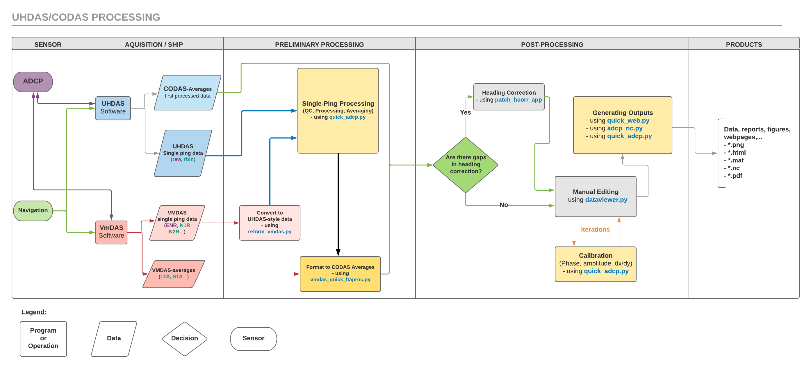
These two diagrams illustrate the workflow behind the CODAS Processing:
this one reads left-to-right (click on the image to expand)
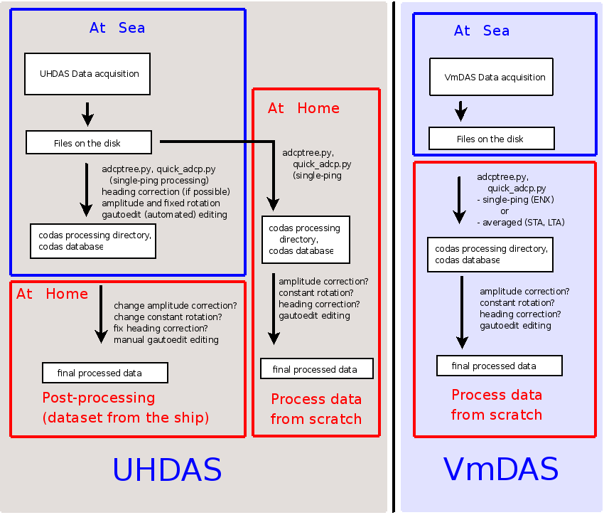
this one reads top-to-bottom
(Return to TOP)
2.1.1. Preliminary Processing
This could refer to re-running the single-ping processing on UHDAS single-ping data with newer algorithms or different settings, or for any CODAS processing of VmDAS data (ENR, LTA, or STA).
In this stage, quick_adcp.py is typically called with a control file with parameters it needs to know for processing, and typically can only be run once.
Pre-averaged data
For PINGDATA and VmDAS LTA or STA data, very little single-ping editing is done prior to averaging. We simply translate these files, whatever their source, and load them into the CODAS database.
Once the first pass is complete, none follows up with the same combination of editing and calibration referred to as Post-processing.
Single-ping data:
The strategy for VmDAS single-ping processing is to use the VmDAS single-ping data (i.e. the ENR data and ancillary inputs such as attitude and position from N1R, N2R, N3R) and:
convert these components into UHDAS-style directories and files
process using the UHDAS+CODAS tools
Single-ping processing of UHDAS (or UHDAS-style) data means:
read the ADCP and ancillary serial data
find UTC time, add position and heading
edit out bad single-ping velocities
average the single-ping data; write to disk.
Reasons for redoing Single-ping Processing of ADCP data:
take advantage of newer tools or algorithms
the cruise was broken into several legs (rejoin the segments)
better final product for VmDAS data (compared to LTA or STA)
bug fixed
something broke during the cruise (the processing failed or a critical ancillary data feed was missing) – see this link for more details about regenerating UHDAS data components.
Algorithmic note: Heading Correction
obtain a heading correction for the gyro headings, using an accurate (preferrably gps-based) attitude device. Examples of accurate GPS-based heading devices include POSMV and Seapath (which also leverage inertial calculations), and Ashtech devices (such as the older ADU5, with 4 antennas, or ABXTWO with 3 antennas)
check the health of the accurate heading device
If there are two heading devices, we use one as a reliable heading (usually a gyro) and the more accurate one as a correction to the reliable one. This is typically applied once, but if there are gaps (eg. during at-sea processing) one may need to “patch” (interpolate) the heading time series.
(Return to TOP)
2.1.2. Post-Processing
Post-processing describes the steps needed after ADCP Data have gone through the steps to get it into a CODAS database. That database exists in an ADCP (sonar) processing directory.
This “existing CODAS database” could have come from at at-sea UHDAS preliminary processing directory, or putting VmDAS LTA (or STA) data into a CODAS framework. Note that loading VmDAS LTA data into a CODAS database is only staging it or post-processing; LTA data are already averaged.
In this stage, the “navigation”, “calibration” and “export” steps described below, all call
quick_adcp.pywith the argument--steps2rerun. These steps can be run multiple times.Patching
if there are gaps in the timeseries of heading correction, one would have to fill these gaps using interpolation, filtering, smoothing and others data manipulation.
patch_hcorr.py has been designed for that purpose.
Navigation
find and smooth the reference layer
Calibration
determine preliminary angle and amplitude calibrations from watertrack and/or bottom track data (using corrected headings)
if large corrections are required, do that before editing
Editing
editing (bottom interference, wire interference, bubbles, ringing, identifying problems with heading and underway bias),
Calibration (check)
final calibration based on edited data
watertrack and bottomtrack calibration, give phase and scale factor
transducer-gps horizontal offset
Documentation
leave notes so someone can see what was done or reproduce the processing steps if necessary
Export
data can be exported in Matlab or NetCDF format
Plot
A simple web-figure generator exists and is useful for distribution and a basic quick look at the data
(Return to TOP)
2.1.3. Practical Processing Guidelines
- (1) Keep data separate from processing:
helps separate “backing up data” (large volume, rarely changes) from “backing up processing” (smaller volume, changes often)
- (2) Do not alter the original data:
if you are going to remake any UHDAS data (rbins or gbins), move the original directory to another name, eg.
mv gbin gbin.orig. If you are usingadcp_database_maker.py, it will do this for you.
Note
When working with UHDAS data from a cruise, leave all the directories the way they were when they came from the cruise. DO NOT replace the “proc” directory with your own processing. Make a new processing directory, somewhere NOT in the data directory.
(3) Keep notes
In your work area, make a directory with your cruise name. This is referred to as the project directory and is usually associated with a cruise.
For any processing you do, start a text file to keep notes. Your notes should include enough information for someone else (or you, months or years later) to understand what was done, including
metadata information about the cruise (eg. instrument settings, serial devices present and what was used)
contents of control files written
steps taken
Your audience should be “yourself in 1 year” if you had to go back and do it again, or explain to someone what you did.
After quick_adcp.py has finished its first run or after using adcp_database_maker.py in the processing directory there will be a text file called cruise_info.txt which you can insert into your text file. This is illustrated in the demos.
Note
It is recommended that your notes sit outside the processing directory. The processing examples illustrate this.
Keeping your notes outside the processsing directory is good insurance, in case you have to delete the processing directory and start over (it does happen) or if you decide to process again with different settings.
If you do have to redo the processing for some reason, it is not a waste of time:
You can verify that your notes are accurate, by using them again
It should be faster the second time
You will learn better the second time
(Return to TOP)