2.4.3. LTA Postprocessing Demo

Note

Directory Strategy

To simplify the documentation, these instructions assume you have set up your directories as in Directory Setup and you are doing your processing demos in my_adcp_py3demos/adcp_pyproc

your practice directory                 source
-----------------------                -----------

my_adcp_py3demos
my_adcp_py3demos/adcp_pyproc                 (new, WORKING IN HERE)
my_adcp_py3demos/uhdas_data                  copy of adcp_py3demos/uhdas_data
my_adcp_py3demos/vmdas_data                  copy of adcp_py3demos/vmdas_data
my_adcp_py3demos/uhdas_style_data            (new, empty, for VmDAS conversion)

---

Scenario:

You want a nice-looking LTA dataset.

To get the most out of this example, you should have already gone through the CODAS post-processing demo. In both cases you are working with data that is already averaged, so there are many things you cannot do. LTA processing is just “converting the LTA files into CODAS averages” followed by “CODAS post-processing”, so definitely be familiar with the post-processing example.

Resources

• command-line help: quick_adcp.py --commands ltapy

• text file (with metadata) from an actual processing directory This file narrates the steps in the manual LTA processing, including postprocessing.

• dataviewer.py documentation (viewing and editing)

• the rest of this web page

Directory Strategy

Preliminary processing has already been done, using one of the following schemes:

• adcp_database_maker.py

• vmdas_quick_adcp.py

• manual steps: vmdas_info.py and adcptree.py

Start making notes

Keep your notes in a file adjacent to the newly created processing directory. For this illustration, the text file will be called os75bb_LTA_postproc.txt.

The processing directory for this example will be os75bb_LTA, the one created by adcp_database_maker.py

---

Note

Everything below here is post-processing. You can look at another example in the UHDAS post-processing demo.

---

We are doing this work in the preliminary processing directory created by adcp_database_maker.py but it could be any of the LTA CODAS processing directories.

Start by going to the vmdas project directory:

cd ~/my_adcp_py3demos/adcp_pyproc/ps0918_vmdas
pwd

The result should be:

/home/adcpproc/my_adcp_py3demos/adcp_pyproc/ps0918_vmdas

Useful Extra step: copy this entire processing directory “as it stands” (with no changes) so we can compare our final product to this original LTA data, for example call the copy os75bb_LTA_orig. You can do that on the command-line before we start. In the ps0918_vmdas project directory, run this command:

cp -a os75bb_LTA  os75bb_LTA_postproc

Now there are two processing directories. We will compare them later.

• os75bb_LTA

• os75bb_LTA_postproc

Last but not least, start a text file with notes:

emacs os75bb_LTA_postproc.txt &

Now change directories into the CODAS processing directory os75bb_LTA_postproc for the rest of the post-processing:

cd os75bb_LTA_postproc

1. DISCOVERY

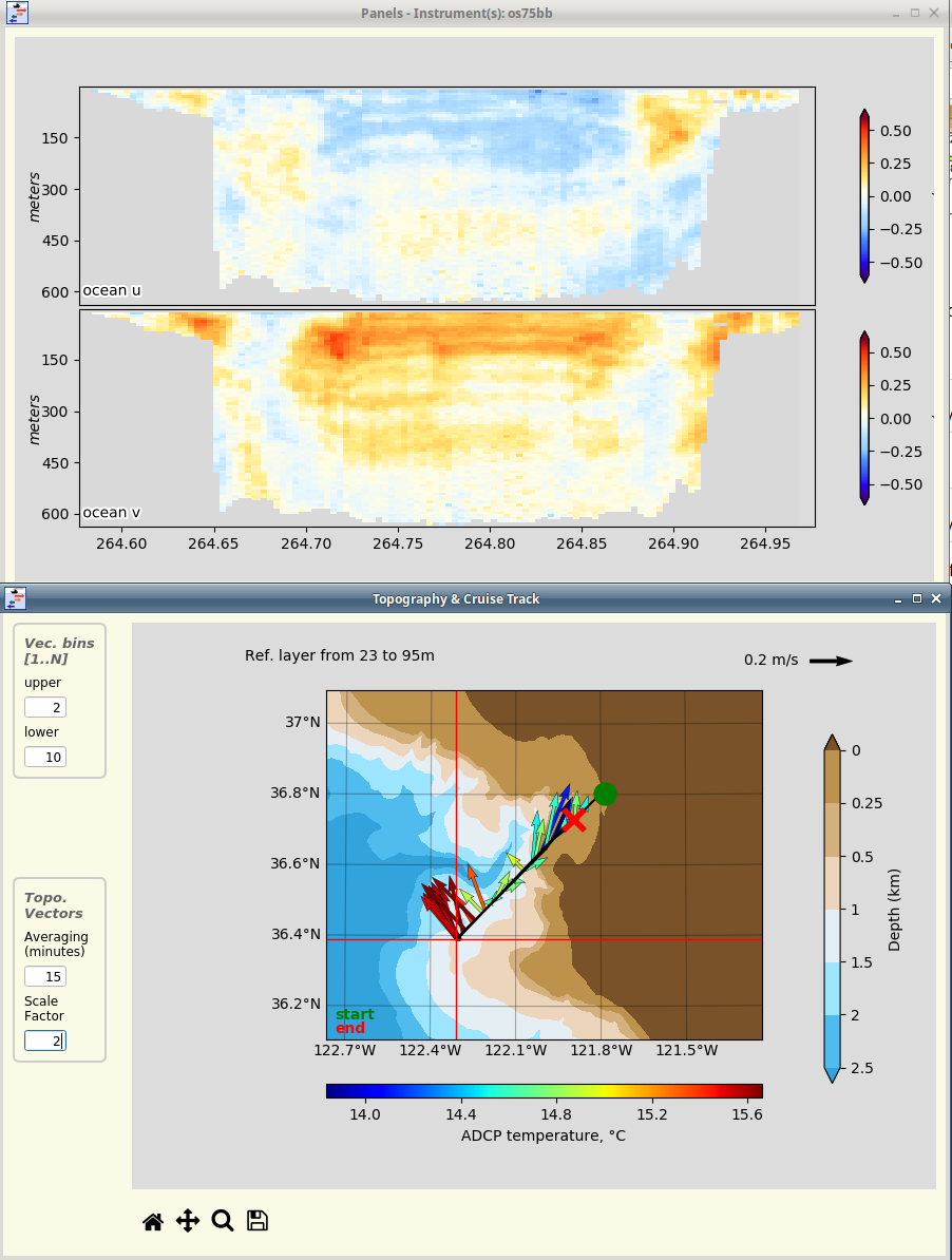
Make a cruise track to see what to expect. We are still in the os75bb_LTA_postproc directory.

Make a cruise track plot:

plot_nav.py nav/aship.gps

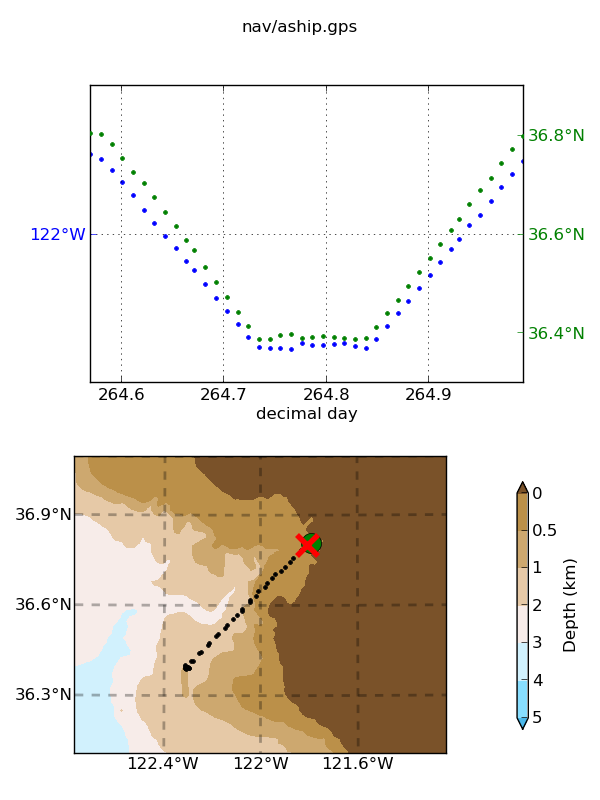
2. PLOTS

Run this command to look at all the plots:

figview.py

You are looking for

• glitches in heading

• gaps in the data

• issues with calibration

3. CHECK CALIBRATION

This is a short out-and-back cruise; probably no watertrack calibration data, vmdas_info.py showed that there is bottom track data. Even though it is a reciprocal track, the cruise is coastal (strong currents) and takes too much time (too large a fraction of a tidal cycle) to use the reciprocal track for calibration.

Note

HINT: The CODAS virtual machine has three little Python programs to speed up the discovery process looking at the calibrations. You can type these shortcuts to look at the calibrations, which really speeds things up.

shortcut:      looking for             what it does (but prettier)
--------       ------------          -----------------------------
catwt.py       watertrack cal        tail -20  cal/watertrk/adcpcal.out
catbt.py       bottomtrack cal       tail -6 cal/botmtrk/btcaluv.out
catxy.py       ADCP-gps offset       tail -6 cal/watertrk/guess_xducerxy.out

check calibration:

**bottomtrack**

------------
unedited: 36 points
edited:   33 points, 2.0 min speed, 2.5 max dev
           median     mean      std
amplitude   0.9998   0.9998   0.0025  <==== no change needed
phase       1.3538   1.5970   0.5428  <==== probably apply 1.5
------------


**watertrack**
Number of edited points:   2 out of   2
  amp   = 1.0040  + 0.1053 (t - 264.8)
  phase =   1.42  + 15.5789 (t - 264.8)
            median     mean      std
amplitude   1.0040   1.0040   0.0085
phase       1.4200   1.4200   1.2558    <=== "consistent" given
                                             that we only have 2 points

So ‘yes’, bottom track; not much watertrack, but it is at least consistent.

Look at the bottom track calibration figure. Note that the phase offset is DIFFERENT on the outbound and inbound legs: That means this dataset was collected using an inaccurate heading device (gyro) so it really needs to be reprocessed with the Ashtech (accurate heading device) used for heading.

4. DATAVIEWER

Look at the data

dataviewer.py

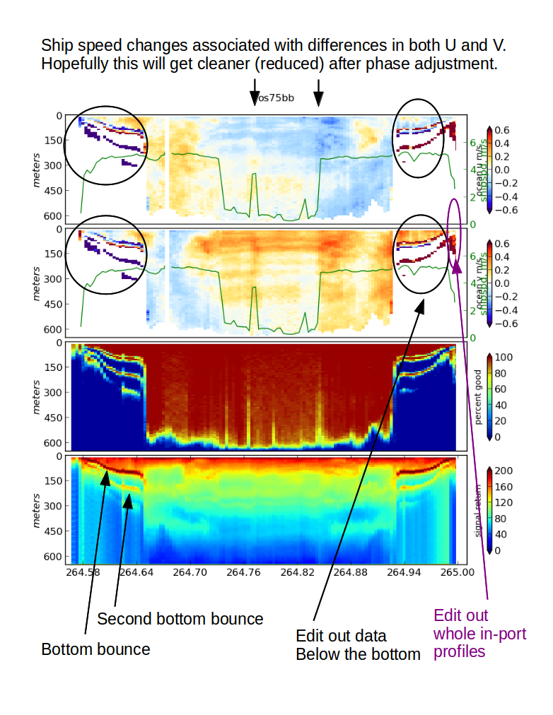
Adjust the phase calibration first.

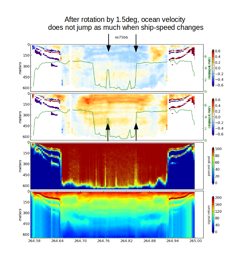
Apply rotation correction (no scale factor necessary):

quick_adcp.py --steps2rerun rotate:navsteps:calib --rotate_angle 1.5  --auto

Check calibration again:

  **bottomtrack**
  ------------
  unedited: 36 points
  edited:   33 points, 2.0 min speed, 2.5 max dev
              median     mean      std
  amplitude   0.9994   0.9997   0.0026
  phase      -0.1377   0.0942   0.5405


This is "close enough" to allow editing at this point

Now look again with dataviewer. The ‘jumps’ at the two arrows are either gone or at least more subtle.

You can also see the vectors are agreeing better:

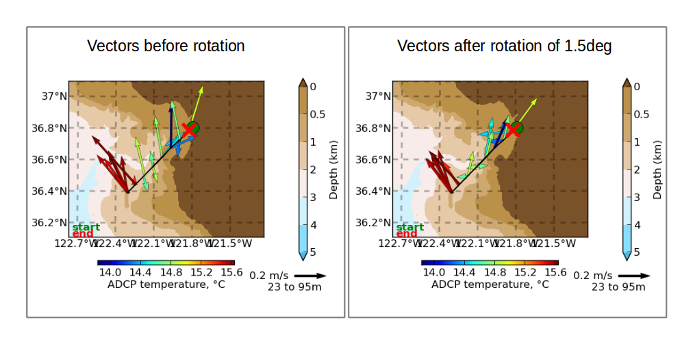
5. EDITING

Now edit out any bad data. See dataviewer.py documentation

Edit bad data:

dataviewer.py -e

Apply editing:

quick_adcp.py --steps2rerun apply_edit:navsteps:calib  --auto

Now look again at the final data:

6. COMPARE

Now can compare them (before and after) by running the following command:

cd ..
dataviewer.py -c  os75bb_LTA os75bb_LTA_postproc

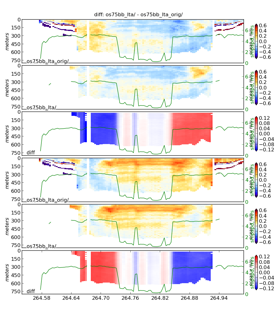
Notice the 10-12cm/s difference in the ocean velocity during the transit legs: that comes from the 1.5deg rotation. The effect of editing is obvious.

Note

Rule of thumb: 1 deg heading error causes a 10cm/s cross-track error in ocean velocity.

---

We’re near the end of the processing for this dataset now.

Review the data:

• Check calibration one more time (look in cal/botmtrk/btcaluv.out)

• Look at the figures again: figview.py --type png

• Check editing again (dataviewer.py)

• Add comments to your processing documentation about

  • interesting features, problems

  • final (complete) calibration values used

7. DATA PRODUCTS

• web plots

• netCDF files

• matlab files

Now make web plots with quick_web.py:

make web plots:

cd os75bb_LTA_postproc
quick_web.py --interactive

If you get a complaint about “already exists”, then you can just update the figures with:

quick_web.py --redo

View with a browser, look at webpy/index.html:

firefox webpy/index.html

When you’re satisfied, extract the data for other people to use.

Data Products

extract matlab data:

quick_adcp.py --steps2rerun matfiles --auto

The matlab files created are

• vector/vector_uv.mat, vector/vector_xy.mat

• contour/contour_uv.mat, contour/contour_xy.mat

• contour/allbins_*.mat

The contents of these matlab files and the netCDF file we generate are documented (See here in the CODAS documentation, in the section concerning ways to access ADCP data.

For this cruise, to get a NetCDF file contour/os75bb.nc run this command:

adcp_nc.py adcpdb contour/os75bb ps0918_demo os75bb --ship_name Point Sur

To check netcdf file:

ncdump -h contour/os75bb_short.nc

---

Note

CODAS processing uses zero-based decimal days. See CODAS Conventions

---

Note

When you are done with all the processing, with permission from the Principal Investigator, we encourage you to submit the data to the Joint Archive for Shipboard ADCP so you get credit for your data collection and processing, and other people can use it too.

Available Demos

• Post-processing a UHDAS dataset

• adcp_database_maker.py

  • Reprocessing UHDAS data with adcp_database_maker.py

  • LTA Processing with adcp_database_maker.py

  • Post-processing LTA data

  • ENR processing with adcp_database_maker.py

• commandline details

  • UHDAS Single-ping Commandline

  • LTA processing: automated command-line

  • LTA command-line processing

  • ENR Single-ping Command Line