2.5.4. ENR Single-ping Command Line

Scenario

You need to process some ENR data (i.e. single-ping level data) and for some reason you need to get into the weeds and edit files, or maybe you just want to know what is happening behind the scenes. This section describes the steps behind adcp_database_maker.py for ENR files.

In general, it is recommended to use adcp_database_maker.py if that is possible.

Resources

• command-line help: quick_adcp.py --commands enrpy

• text file (with metadata) from actual processing directory

• dataviewer.py documentation (viewing and editing)

• the rest of this web page

---

Preliminary processing of ENR data requires that the VmDas data be evaluated (to discover the possible position and heading feeds, and learn about the ADCP). Using the results of that discover, the VmDAS data are “converted” to “uhdas-style data”. After that, the steps are similar to single-ping processing of UHDAS-style data. The steps are:

(Stage 1) Discovery

1. Set up Project Directory

2. Get information about the VmDAS data

(Stage 2) Conversion to UHDAS-style data:

1. create a configuration file that associates the serial source files (N1R/*rbin) with the types of messages that need to be extracted (for heading, position, etc).

2. use the configuration file to make “UHDAS-style data”:

   • STAGING:

     • extract the serial messages from the ancillary (N1R, N2R, N3R) files to create rbins with position or heading information (this is done in the VmDAS data directory)

   • CONVERTING:

     • (i) chop up the ENR files into files with UHDAS_naming convention where a new file is started to keep files less than 2-hour chunks, and any time configuration changed (eg. bottom track ON/OFF)

     • (ii) chop up the N1R/*rbin, N2R/*rbin files to match the time ranges and file convention of the new UHDAS raw data

(Stage 3) Preliminary Processing:

At this stage, we’re back to the UHDAS single-ping processing steps. The only difference is that this ship was not running UHDAS so we’ve had to guess or infer everything about it.

1. set up a configuration file that controls the processing parameters related to the installation (eg. position source, heading source)

2. create a CODAS processing directory using the configuration file from (3a)

3. create a control file (q_py.cnt) within the CODAS processing directory which controls parameters related to this ADCP data and its pings (eg. averaging length, pingtype)

4. run quick_adcp.py

Then you are back to post-processing.

---

2.5.4.1. Instructions

2.5.4.1.1. Make some directories, get information

Note

Directory Strategy

To simplify the documentation, these instructions assume you have set up your directories as in Directory Setup and you are doing your processing demos in my_adcp_py3demos/adcp_pyproc

your practice directory                 source
-----------------------                -----------

my_adcp_py3demos
my_adcp_py3demos/adcp_pyproc                 (new, WORKING IN HERE)
my_adcp_py3demos/uhdas_data                  copy of adcp_py3demos/uhdas_data
my_adcp_py3demos/vmdas_data                  copy of adcp_py3demos/vmdas_data
my_adcp_py3demos/uhdas_style_data            (new, empty, for VmDAS conversion)

---

These are the commands that will be run during Stages 1,2 and 3:

Steps	program to run	what it creates
Step 1 Discovery about VmDAS data	vmdas_info.py	files with serial and ADCP information
Step 2 Conversion to UHDAS-style data
(2a) make config file for N1R and ENR conversion	reform_vmdas.py	config/reform_defs.py config/vmdas2uhdas.py
(2b) convert vmdas data to uhdas-style	config/vmdas2uhdas.py
Step 3 Preliminary Processing
(3a) configuration for processing	proc_starter.py	config/CRUISE_proc.py
(3b) create a CODAS processing directory	adcptree.py	CODAS processing directory
(3c) create q_py.cnt	(use an editor)	q_py.cnt
(3d) run the preliminary processing	quick_adcp.py	CODAS database and supporting files

2.5.4.1.2. (Stage 1) Get information from VmDAS data

Note

If you have not already processed UHDAS single-ping data using Python, you should go do that now. The whole point of “Stage 2” is to create UHDAS data and a configuration file to process the data. That is the same as “step 1” in UHDAS processing, but we have to do more here. So be sure you are familiar with UHDAS single-ping processing. The instructions are here.

Note

We start work in the project directory so ensure that you have a project directory.

Start here:

cd ~/my_adcp_py3demos/adcp_pyproc
pwd

The result should be:

/home/adcpproc/my_adcp_py3demos/adcp_pyproc

---

1. If you have not done it yet, create a project directory to hold all our information about this cruise.

mkdir ps0918_vmdas

Then change directory.

cd ps0918_vmdas

Now start keeping notes and assembling information in this project directory. Since we will be processing os75bb data, the example filename is ps0918_vmdas/os75bb_manual_enr.txt.

2. Get information about the LTA files; store the information in ps0918_vmdas:

First check that we are in the project directory

pwd

Should return:

/home/adcpproc/my_adcp_py3demos/adcp_pyproc/ps0918_vmdas

Now get the information:

vmdas_info.py --logfile  lta_manual_info.txt  os ../../vmdas_data/ps0918/*LTA

Look at that information:

cat lta_manual_info.txt

Now we have this:

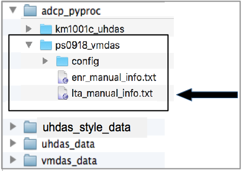
You can also get a little more information about the raw files:

vmdas_info.py --logfile enr_manual_info.txt  os ../../vmdas_data/ps0918/*ENR

Click here to see an annotated version of the file lta_manual_info.txt and the locations where the following information are found:

• these are ‘bb’ pings

• transducer angle was 1.18

• N1R is a gyro (primary heading) message name is “hdg”

• N2R is an Ashtech (heading correction) message name is adu

• N3R is a GPS (positions)

---

2.5.4.1.3. (Stage 2) Convert VmDAS to UHDAS-style

Note

Now we move to the project directory ps0918_vmdas

1. If you don’t already have one, make a ‘config’ directory inside ps0918_vmdas

mkdir config

We will run reform_vmdas.py on the command line in the project directory. The arguments are described below:

 #option and value                      # what it is

--project_dir_path ./                     # identify the project directory
--vmdas_dir_path ../../vmdas_data/ps0918  # path to VmDAS data
--uhdas_style_dir  ../../uhdas_style_data # where uhdas-style data is created
--cruisename ps0918                       # used for uhdas-style data and filenames

Here is the command to run. If you are following the directory structure for the demo, just copy and paste this in a command-line terminal:

reform_vmdas.py --project_dir_path ./ --vmdas_dir_path ../../vmdas_data/ps0918 --uhdas_style_dir ../../uhdas_style_data  --cruisename ps0918_manual --start ..

---

A gui pops up, with all entries pre-filled.

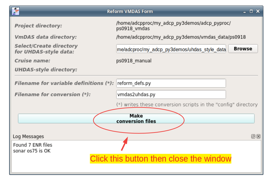
Click the blue button, then close the window.

---

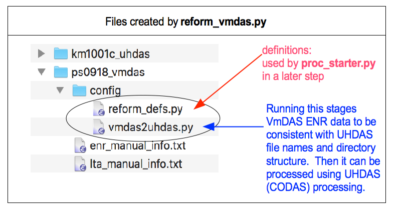
The purpose of this program is to create two files:

1. a file with variable names for future steps (config/reform_defs.py)

2. a program to run next (to convert vmdas data to uhdas data, config/vmdas2uhdas.py)

The directory now looks like this:

Now we are ready to actually do the conversion. Transform VmDAS data into UHDAS data by running this comand now:

cd  config
python3 vmdas2uhdas.py

This command

1. creates N1R, N2R, N3R directories in the vmdas_data directory (shown here)

2. recasts the OS75 ENR data and the N1R, N2R, N3R as UHDAS data in the uhdas_style_data/ps0918_manual directory (shown here).

---

2.5.4.1.4. (Stage 3) Preliminary Processing

Finally, run the following program, which will create the processing configuration file for your new UHDAS-style data. You need to specify the file made in Stage 1 that stored the variables. By default it is called reform_defs.py (see where it was written).

Run this from inside the “config” directory::

proc_starter.py reform_defs.py

This creates another GUI with boxes to fill in. Use information from lta_manual_info.txt and this guide.

Now fill in (or alter) the boxes:

• transducer angle

• transducer depth

• (position feed is OK)

• heading should come from the gyro (N1R)

• Enable heading correction

• heading correction should come from the Ashtech (N2R)

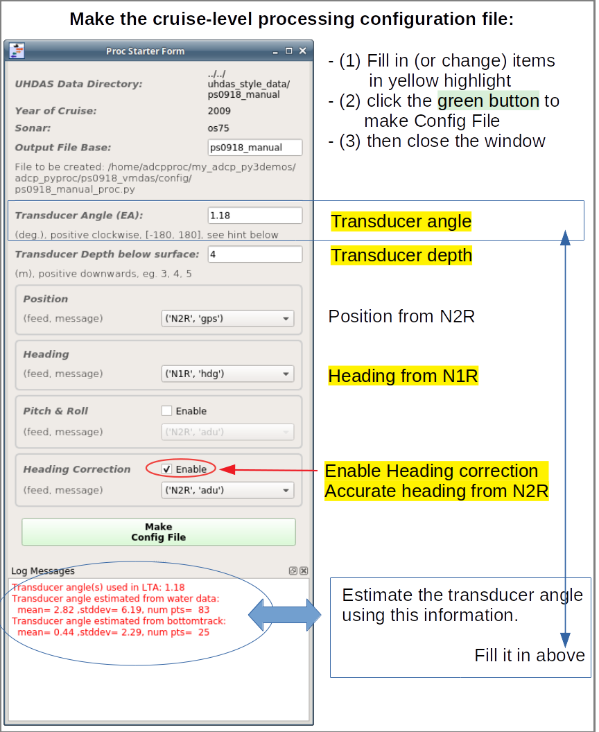
Then click the green button and close the window.

The program creates a correctly-formatted file suitable for processing UHDAS single-ping data. In this example, the file is ps0918_manual_proc.py.

---

Now everything is set up for UHDAS single-ping processing

---

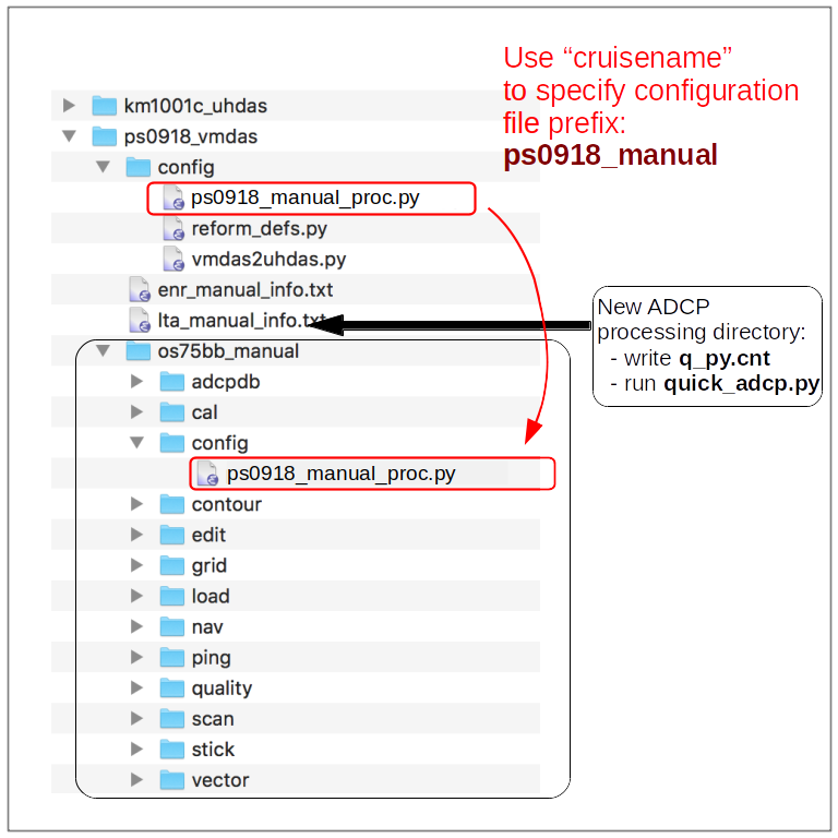
1. Run adcptree.py to make the processing directory

   In the terminal, go back one directory to “ps0918_vmdas” and make the OS75 ENR processing directory:

   You must use the same prefix here that is specified above: in this example ps0918_manual.

cd ..
adcptree.py os75bb_manual --datatype uhdas --cruisename ps0918_manual
cd os75bb_manual

If your command-line terminal has this text, you are ready for the next step:

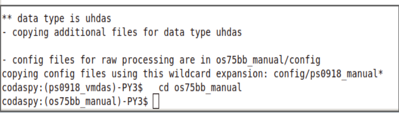
Warning

Do not proceed if you do not have os75bb_manual/config/ps0918_manual_proc.py If you do not have this file, check the cruisename specified when calling adcptree.py.

Here is where the configuration file landed inside the processing directory:

---

2. Make the q_py.cnt control file in the processing directory:

   Change directories to ADCP processing directory (os75bb_manual) and make the quick_adcp.py control file

First check where we are:

pwd

This should give us:

/home/adcpproc/my_adcp_py3dems/adcp_pyproc/ps0918_vmdas/os75bb_manual

The contents of q_py.cnt:

### q_py.cnt contents

## python processing

 --yearbase 2009             ## required, for decimal day conversion
                             ##     (year of first data)
 --cruisename ps0918_manual  ## *must* match prefix in config dir
 --dbname aship              ## database name; in adcpdb.  eg. a0918
                             ##
 --datatype uhdas            ## datafile type
 --sonar os75bb              ## specify instrument letters, frequency,
                             ##     (and ping type for ocean surveyors)
 --ens_len  300              ## averages of 300sec duration
                             ##
 --update_gbin               ## required for this kind of processing
 --configtype  python        ## file used in config/ dirctory is python
                             ##
 --ping_headcorr             ## ps0918_manual_proc.py says use HDT first,
                             ##    correct to ashtech
 --max_search_depth 1500     ## try to identify the bottom and eliminate
                             ##    data below the bottom IF topo says
                             ##    the bottom is shallower than 1000m

There is also a linux shortcut for making a file from the commandline. Just follow instructions and copy the right part of the hint and paste it into the command-line terminal.

---

3. run quick_adcp.py:

quick_adcp.py --cntfile q_py.cnt  --auto

---

The rest of the steps are the same as post-processing:

• keep notes: add “cruise_info.txt” and annotate

• patch heading correction (if necessary)

• check calibration

• edit

• check calibration (again)

• check editing

• make web plots

• compare with LTA processing

These steps are laid out in all the other demos, and should be practically identical to lta processing after running quick_adcp.py.

---

ADDITIONAL NOTES

Given that you previously did the LTA demo and thus that os75bb_LTA exists along side with os75bb_manual and after phase calibration of both LTA and single-ping processing, one can compare the two datasets using the following command:

cd ..
dataviewer.py -c os75bb_manual/ os75bb_LTA/

(See this link for further details on the comparison mode in dataviewer.py)

You will notice the following differences made by single-ping processing:

• additional is bias removed by using accurate heading (heading correction)

• bottom reflections are mostly gone in the single-ping velocities (panels 1 and 4)

• LTA data still has bottom interference (panels 2 and 6)

• remaining differences come in two flavors:

  • velocities are more stable in single-ping processing (more variable in deep water in LTA data). This is due to the single-ping editing done with the ENR (uhdas-style data) processing

  • There is a 2-6cm/s bias in the LTA data due to the use of gyro as the heading device. This is corrected in the single-ping processing

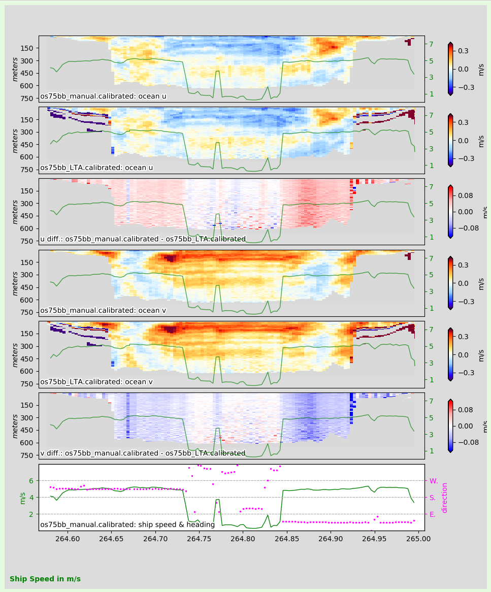
It is worth the trouble to do the ENR processing

---

Note

CODAS processing uses zero-based decimal days. See CODAS Conventions

---

Note

When you are done with all the processing, with permission from the Principal Investigator, we encourage you to submit the data to the Joint Archive for Shipboard ADCP so you get credit for your data collection and processing, and other people can use it too.

Available Demos

• Post-processing a UHDAS dataset

• adcp_database_maker.py

  • Reprocessing UHDAS data with adcp_database_maker.py

  • LTA Processing with adcp_database_maker.py

  • Post-processing LTA data

  • ENR processing with adcp_database_maker.py

• commandline details

  • UHDAS Single-ping Commandline

  • LTA processing: automated command-line

  • LTA command-line processing

  • ENR Single-ping Command Line