2.5.2. LTA processing: automated command-line

Note

Directory Strategy

To simplify the documentation, these instructions assume you have set up your directories as in Directory Setup and you are doing your processing demos in my_adcp_py3demos/adcp_pyproc

your practice directory                 source
-----------------------                -----------

my_adcp_py3demos
my_adcp_py3demos/adcp_pyproc                 (new, WORKING IN HERE)
my_adcp_py3demos/uhdas_data                  copy of adcp_py3demos/uhdas_data
my_adcp_py3demos/vmdas_data                  copy of adcp_py3demos/vmdas_data
my_adcp_py3demos/uhdas_style_data            (new, empty, for VmDAS conversion)

---

Scenario:

You need a quick look at one or many VmDAS cruises to evaluate quality, settings, location, potential, and try to assess the amount of work necessary to bring the cruise in to some useful form of ocean current data.

It is also prefectly reasonable to actually start the LTA processing with this mechanism.

Note

This is what adcp_database_maker.py is actually running when it does LTA or STA processing.

Resources

• command-line help: vmdas_quick_ltaproc.py --help

• text file (with metadata) from an actual processing directory This file narrates the steps in the manual LTA processing, including postprocessing.

• dataviewer.py documentation (viewing and editing)

• the rest of this web page

This program runs on the command-line. You can run it for many collections of LTA files.

To replicate what adcp_database_maker.py is doing, run the command (below) from the adcp_pyproc directory, and point to the ps0918_vmdas project directory in the command-line.

The arguments mean:

option name               option value          what it does
------------              -------------         --------------
--cruisename              ps0918_quicklta      prefix for "info" and "proc" files
--procroot                ps0918_vmdas         project directory (put files
                                                  and processing directory here)
--procdir                 os75bb_quicklta      processing directory name

First, make sure we are in the right directory:

cd ~/my_adcp_py3demos/adcp_pyproc
pwd

The result should be:

/home/adcpproc/my_adcp_py3demos/adcp_pyproc

Now run this command:

vmdas_quick_ltaproc.py --cruisename ps0918_quick --procroot ps0918_vmdas --procdir os75bb_quicklta  ../vmdas_data/ps0918/*LTA

Then you will have identical files and directories to the previous section (adcp_database_maker.py) but the names will be different.

---

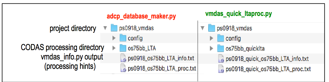
Here is what it does:

1. DISCOVERY: find information about the data

The program will run vmdas_info.py (as in the next demo) and will write the results in a file. It narrates as it goes along:

using cruisename "ps0918_quick"
- will deduce yearbase
- if there are multiple EA or multiple ensemble time durations:
   - will stop.  use "--force" to override
processing will take place in ps0918_vmdas/os75bb_quicklta
- will deduce sonar
  found sonar os75bb
  Sonar:  os75bb
Writing additional information to logfile ps0918_vmdas_os75bb_LTA_info.txt:
- determining summary information about LTA data files
- sorting files in time order
- guessing instrument model
- about to guess EA from raw data files...
- determining ensemble length from LTA files
- guessing additional information for single-ping processing)
- guessing heading source
- trying to determine serial NMEA messages
found one consistent ensemble length: using 299sec

We specified the cruise as ps0918_vmdaslta so the program writes the vmdas_info.py output in ps0918_vmdas_os75bb_LTA_info.txt.

2. LOADING THE DATABASE

The program then creates a processing directory and writes out the q_py.cnt control file with the information it found above. Then it runs quick_adcp.py to create the processed data, and narrates as it goes along:

adcptree created ps0918_vmdas/os75bb_quicklta
wrote ps0918_vmdas/os75bb_quicklta/q_py.cnt
running: quick_adcp.py --cntfile q_py.cnt --auto
done with quick_adcp.py
wrote cals.txt

3. DATA PRODUCTS

Data products are created so you can take a quick look at the data:

Making web site with figures using "quick_web.py"

netCDF files:
-------------:
- made short netCDF file contour/os75bb.nc
- netCDF variables are defined in contour/CODAS_netcfd_variables.txt
- CODAS processing described in contour/CODAS_processing_note.txt

You can test the netCDF file by typing:

ncdump -h ps0918_vmdas/os75bb_quicklta/contour/*nc

You can browse the web site with:

firefox  ps0918_vmdas/os75bb_quicklta/webpy/index.html

4. CALIBRATION

Calibration values are printed to the screen, for easy viewing:

===================================================
Processed 3 os75bb LTA files with 299sec ensemble length

**WATERTRACK**
---------------------------
Number of edited points:   2 out of   2
            median     mean      std
amplitude   1.0040   1.0040   0.0085
phase       1.4200   1.4200   1.2558


**BOTTOMTRACK**
---------------------------
unedited: 36 points
edited:   33 points, 2.0 min speed, 2.5 max dev
            median     mean      std
amplitude   0.9998   0.9998   0.0025
phase       1.3538   1.5970   0.5428

5. METADATA

Files are written with information about the dataset and the processing:

============
=== Data ===
============

- vmdas_info data summary is in this file:
         ps0918_vmdas_os75bb_LTA_info.txt

================
== Processing ==
================

- Summary processing information is in this file:
        ps0918_vmdas/os75bb_quicklta/cruise_info.txt

- Calibrations (also shown above) are summarized in:
        ps0918_vmdas/os75bb_quicklta/cals.txt

5. VIEWING THE DATA PRODUCTS

Figures are made during processing, and a summary “web site” is created for the whole cruise. In addition dataviewer.py can be used to explore the data:

===============
=== Figures ===
===============


To view all figures generated during processing,
        figview.py ps0918_vmdas/os75bb_quicklta
run this command:
(On a Mac, you may need to use this more complicated version:)
        pythonw `which figview.py` ps0918_vmdas/os75bb_quicklta


To explore the dataset, run this command:
        dataviewer.py ps0918_vmdas/os75bb_quicklta
(On a Mac, you may need to use this more complicated version:)
        pythonw `which dataviewer.py` ps0918_vmdas/os75bb_quicklta


To look at the web plots, in a web browser
    open ps0918_vmdas/os75bb_quicklta/webpy/index.html

6. POST-PROCESSING HINTS

Postprocessing still requires calibration and editing. At this stage, you can go to the LTA Postprocessing demo.

======================
=== Postprocessing ===
=====================

all postprocessing occurs in ps0918_vmdas/os75bb_quicklta; change directories first

      cd  ps0918_vmdas/os75bb_quicklta

If warranted, apply a rotation calibration using mean or median
of watertrack or bottom track calibration values.  If mean and
median agreed at 0.5deg, apply as follows, using 0.5 for XXX:

     quick_adcp.py --steps2rerun rotate:navsteps:calib --rotate_angle XXX --auto


After rotation and editing, to remake the netCDF file:

     adcp_nc.py adcpdb/aship contour/os75bb.nc ps0918_vmdas os75bb


After rotation and editing, to remake the webpy web site:

    quick_web.py --redo

Note

Reminder: all this information is written in ps0918_vmdas/ps0918_vmdas_os75bb_LTA_proc.txt

Available Demos

• Post-processing a UHDAS dataset

• adcp_database_maker.py

  • Reprocessing UHDAS data with adcp_database_maker.py

  • LTA Processing with adcp_database_maker.py

  • Post-processing LTA data

  • ENR processing with adcp_database_maker.py

• commandline details

  • UHDAS Single-ping Commandline

  • LTA processing: automated command-line

  • LTA command-line processing

  • ENR Single-ping Command Line