2.5.1. UHDAS Single-ping Commandline

Resources

• command-line help: quick_adcp.py --commands uhdaspy

• text file (with metadata) from an actual final processing directory

• dataviewer.py documentation (viewing and editing)

• the rest of this web page

---

Note

Directory Strategy

To simplify the documentation, these instructions assume you have set up your directories as in Directory Setup and you are doing your processing demos in my_adcp_py3demos/adcp_pyproc

your practice directory                 source
-----------------------                -----------

my_adcp_py3demos
my_adcp_py3demos/adcp_pyproc                 (new, WORKING IN HERE)
my_adcp_py3demos/uhdas_data                  copy of adcp_py3demos/uhdas_data
my_adcp_py3demos/vmdas_data                  copy of adcp_py3demos/vmdas_data
my_adcp_py3demos/uhdas_style_data            (new, empty, for VmDAS conversion)

---

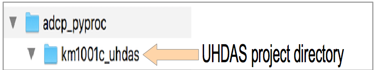
Make a project directory to work on this cruise. This directory will be called km1001c_uhdas, and will hold notes and the individual Processing Directory for each sonar.

Instructions

Note

We start work in the project directory so change directories to that location

cd ~/my_adcp_py3demos/adcp_pyproc/km1001c_uhdas
pwd

The result should be:

/home/adcpproc/my_adcp_py3demos/adcp_pyproc/km1001c_uhdas

---

start making notes: We will be processing the os38nb data, so call the file os38nb_fullproc.txt.

(1) create processing configuration file

In order to perform the preliminary processing, we need to generate a suitable configuration. This resides in the Config Directory, and contains instructions for processing data from this cruise, such as transducer depth, transducer angle and ancillary data sources (heading and attitude). This new file contains modern settings and modern syntax for the specified ship. The settings may be different from the settings that are appropriate for your cruise (eg. an older cruise may have different serial feeds available). So we create a new file, with modern syntax and variable names, and then edit as needed. There is no GUI for this step.

First, verify that we are in the project directory km1001c_uhdas:

pwd

The result should be:

/home/adcpproc/my_adcp_py3demos/adcp_pyproc/km1001c_uhdas

Now we make the config directory to hold cruise-level processing information. Make the directory (if it does not exist) and change directories to go inside:

mkdir config
cd config

This example is a Kilo Moana cruise: km1001c. Make the configuration file and edit for the appropriate cruise name and year. This file is Python code, so be careful about your syntax when you edit the file: leave punctuation and indentation “as is”.

Make the configuration file:

uhdas_proc_gen.py -s km

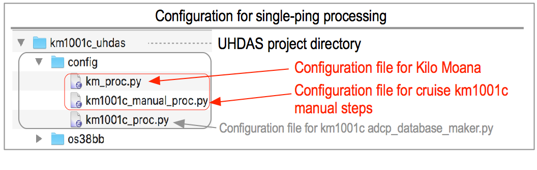
This creates a file called “km_proc.py”

Copy to a new version for our cruise (use the cruisename km1001c_manual):

cp km_proc.py km1001c_manual_proc.py

Edit the file and add these four (4) lines to the top of km1001c_manual_proc.py, for instance:

emacs km1001c_manual_proc.py &

Add these line to the top:

# --- begin section to add ---
# full path to uhdas data directory (do not use relative path)
uhdas_dir = '/home/adcpproc/my_adcp_py3demos/uhdas_data/km1001c'
yearbase = 2010                  # usually year of first data logged
shipname = 'Kilo Moana' # for documentation
cruiseid = 'km1001c'              # for titles
# --- end of section to add ---

Now go back one level to km1001c_uhdas:

cd ..

The contents of km1001c_manual_proc.py is outlined here.

Your new file, km1001c_manual_proc.py has been created using modern syntax, variable names, and recent settings for this ship. The older the dataset you are reprocessing, the more likey there have been changes to the configuration file. The most likely things to have changed are:

• transducer angle

• position instrument

• heading instrument

• heading correction instrument

The original settings are stored in the config directory in the at-sea processing directory (in the proc directory inside the UHDAS data) for the instrument, for example:

my_adcp_py3demos/uhdas_data/km1001c/proc/os38nb/config

The files that were actually used for the preliminary processing ran the generation of code when the cruise took place.

Note

For this demo, there are no substantive differences between then and now.

---

(2) Create the CODAS processing directory

Now create the processing directory. We do this within the UHDAS km1001c project directory, km1001c_uhdas. There may be several CODAS processing directories adjacent to each other, for instance

• postprocessing demo

• UHDAS preliminary processing using adcp_database_maker.py

• UHDAS preliminary processing (using command-line instructions)

---

The “cruisename” argument is used to identify which config/*_proc.py file we will use. By using cruisename=”km1001c_manual” we identify config/km1001c_manual_proc.py as the file we want.

You should be in the project directory, i.e. km1001c_uhdas:

cd ~/my_adcp_py3demos/adcp_pyproc/km1001c_uhdas
pwd

The result should be:

/home/adcpproc/my_adcp_py3demos/adcp_pyproc/km1001c_uhdas

---

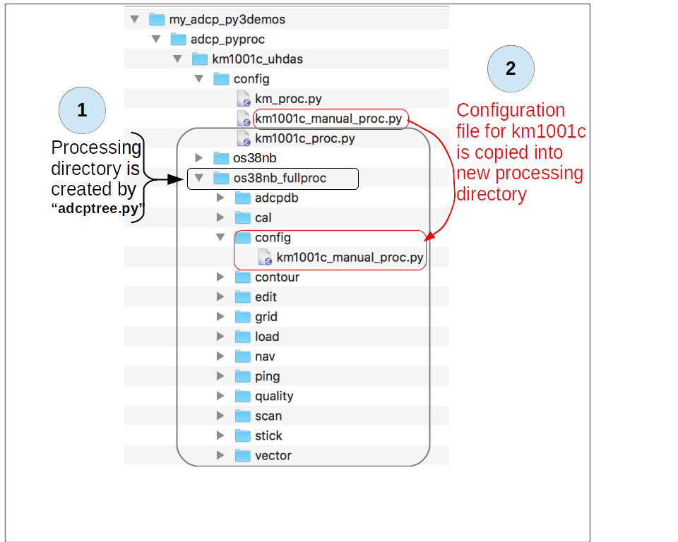
Set up the processing directory by typing:

adcptree.py  os38nb_fullproc --datatype uhdas --cruisename km1001c_manual

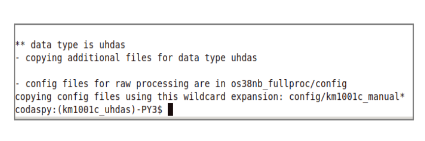
If you are successful thus far, your new adcp processing directory os38nb_fullproc should have a new config directory also with km1001c_manual_proc.py in it. The screen messages from adcptree.py will look like this:

Warning

Do not proceed if you do not have os38nb_fullproc/config/km1001c_manual_proc.py If you do not have this file, check the cruisename specified when calling adcptree.py.

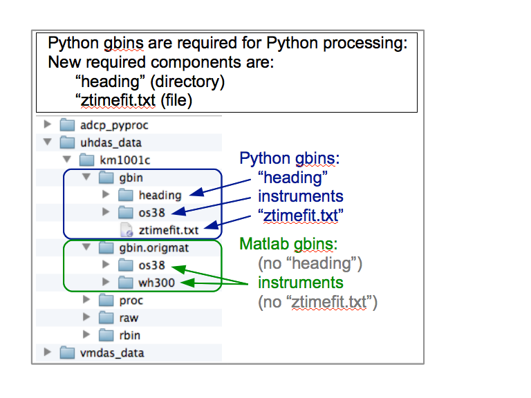
This figure shows where the new config directory lands, and the file in it that will be used for processing:

(3) Create q_py.cnt control file

Now we will make the control file (q_py.cnt) for quick_adcp.py to use in processing. Preliminary processing uses most of the variables that were set up in step (2). There are other parameters which depend on the ADCP model etc, and those are stored in the q_py.cnt file.

During preliminary processing, quick_adcp.py uses --cruisename to find the configuration file config/km1001c_manual_proc.py and reads those values. The control file below sets additional variables.

The rest of the work takes place INSIDE the processing directory

(3a) change directories to the processing directory just created:

cd  os38nb_fullproc

(3b) create a quick_adcp.py control file called: q_py.cnt. This requires

opening the file with an editor and pasting the contents in:

####----- begin q_py.cnt------------
## all lines after the first "#" sign are ignored
 --yearbase    2010
 --cruisename  km1001c_manual   # used to identify configuration files
                         #  *must* match prefix of files in config dir

 --update_gbin   ## NOTE: You should generally remake gbins
             ## - you are not sure
             ## - if parameters for averaging changed
             ## - various other reasons.

             ## ==> MAKE SURE you move the original gbin directory
             ##     to another name first!!  Default directory
             ##     to make gbins is in uhdas_dir


             ## or... alternatively, use this parameter

 --configtype python  ## use km1001c_manual_proc.py for configuration

 --sonar       os38nb
 --dbname      aship
 --datatype    uhdas
 --ens_len     300

 --ping_headcorr        ## applies heading correction.
                    ## this ONLY works if there is a heading
                    ##     correction device specified in the
                    ##     config/km1001c_manual_proc.py file

 --max_search_depth 3000  #if the topography says the ocean is deeper
                      # than this, do not autodetect the bottom.
                      # (reduces likelihood of shallow scattering
                      # layers being identified as the bottom)

In linux you can also use this shortcut, called a “heredoc”.

---

Now we are ready to set and run the single-ping processing. This will also make new gbins. Because we must remake the “gbin” files, YOU MUST RENAME THE ORIGINAL GBIN DIRECTORY to another name, eg gbin.origmat, or quick_adcp.py will fail! First, see what is there:

ls  ../../../uhdas_data/km1001c/

Then rename the gbin directory:

mv  ../../../uhdas_data/km1001c/gbin ../../../uhdas_data/km1001c/gbin.orig
ls  ../../../uhdas_data/km1001c

(4) Run quick_adcp.py to do the preliminary processing

Now run the command to actually perform the preliminary processing:

quick_adcp.py --cntfile q_py.cnt --auto

Note

You can use the --auto option to speed through the preliminary processing and not ask any questions, or if you leave it out, you must answer with ‘yes’ each time, but you get to read the steps being performed.

Note the difference between the old Matlab gbin directory and new Python gbin directory:

---

Everything below here is CODAS Post-processing

---

Check processing:

1. look at all figures (figview.py --type png)

2. look at heading correction: does it need to be patched?

3. look at watertrack and bottom track calibrations: what can we expect?

Figures to look at

directory	files	information
nav	nav_plot.png	cruisetrack
nav	reflayer_*.png	reference layer
edit	temp_plot.png	temperature
edit	nping_plot.png	pings per average
cal/rotate	hcorr_mpl_*.png	heading correction
cal/watertrk	wtcal*.png	watertrack calib
cal/botmtrk	btcal.png	bottomtrack calib

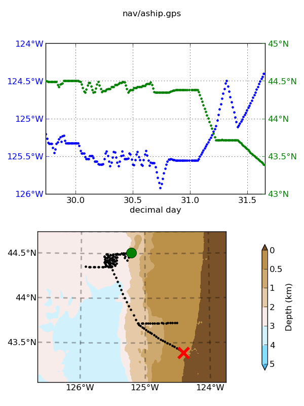
A nicer cruise track plot can be made by running this:

plot_nav.py nav/aship.gps

4. review data

1. heading correction device:

   figview.py cal/rotate/*png
   

Conclude: no action needed : note that in your text file

2. check calibration: (cal/watertrk/adcpcal.out):

   **watertrack**
   ------------
   Number of edited points:  34 out of  35
      amp   = 1.0074  + -0.0033 (t -  30.3)
      phase =   0.05  + 0.1635 (t -  30.3)
               median     mean      std
   amplitude   1.0080   1.0074   0.0064 <== pretty close to 1.0
   phase       0.0900   0.0511   0.4541 <== pretty close to 0.0
   ------------
   

Watertrack calibration indicates calibration is close; we can go ahead and edit without editing out “false anomalies”.

3. look at the data

dataviewer.py

Here is the view:

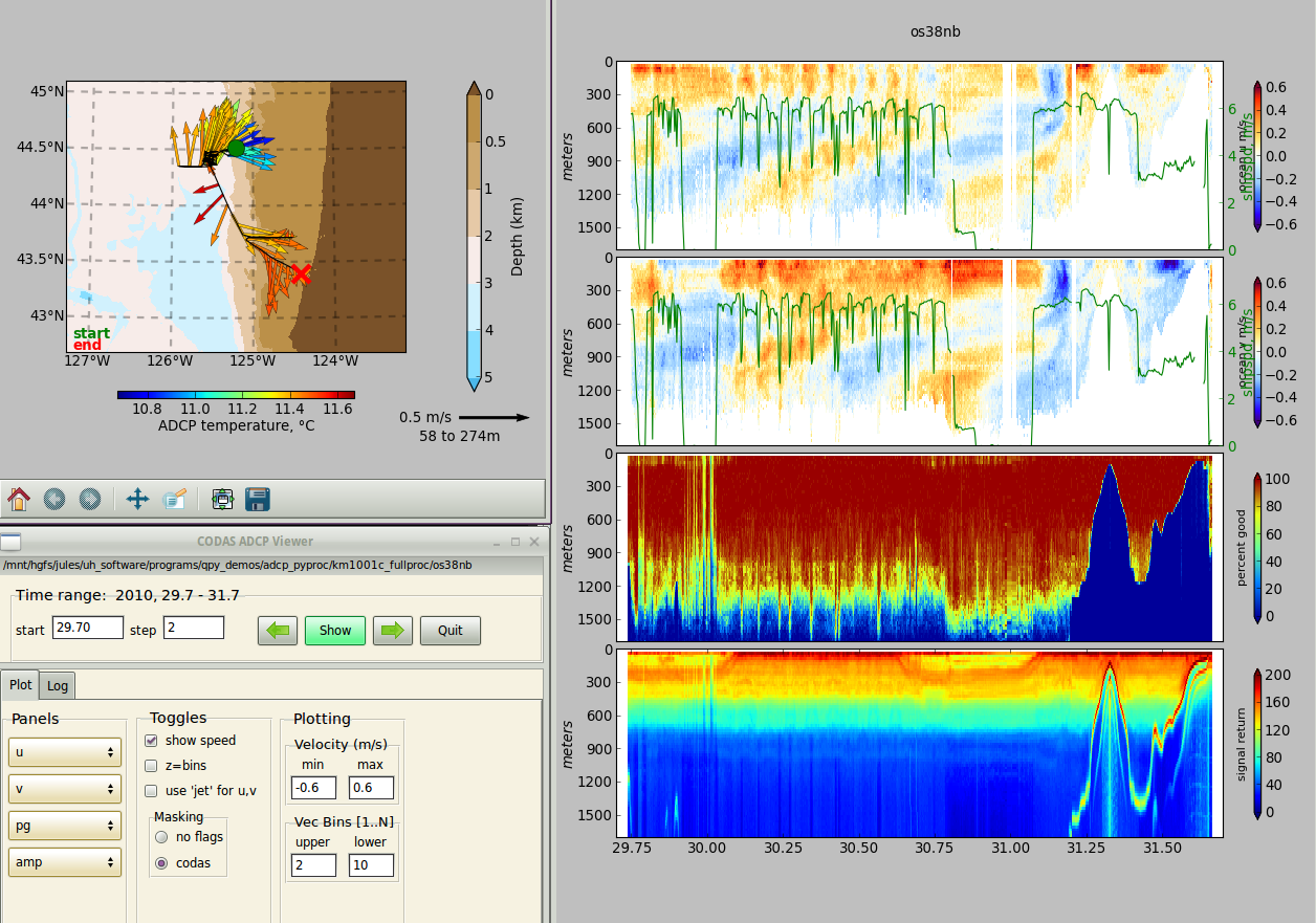
5. Now edit out any bad data. See dataviewer.py documentation

dataviewer.py -e

Apply editing

quick_adcp.py --steps2rerun apply_edit:navsteps:calib  --auto

Now look at everything again.

6. check editing – looks OK

 dataviewer.py


check calibrations again (cal/watertrk/adcpcal.out)::




       **watertrack**
   ------------
   Number of edited points:  34 out of  35
      amp   = 1.0071  + -0.0020 (t -  30.3)
      phase =   0.05  + 0.1809 (t -  30.3)
               median     mean      std
   amplitude   1.0080   1.0071   0.0058
   phase       0.0900   0.0494   0.4431
   ------------

still need scale factor::


 quick_adcp.py --steps2rerun rotate:navsteps:calib --rotate_amplitude 1.007 --auto



check calibrations again (cal/watertrk/adcpcal.out)::

           **watertrack**
   ------------
   Number of edited points:  34 out of  35
      amp   = 1.0001  + -0.0018 (t -  30.3)
      phase =   0.05  + 0.1840 (t -  30.3)
               median     mean      std
   amplitude   1.0010   1.0001   0.0058
   phase       0.0935   0.0496   0.4439
   ------------


phase correction is very small.  Here is how you would apply it::


    quick_adcp.py --steps2rerun rotate:navsteps:calib --rotate_angle 0.06 --auto


check calibration again::


        **watertrack**
    ------------
    Number of edited points:  34 out of  35
       amp   = 1.0001  + -0.0018 (t -  30.3)
       phase =  -0.01  + 0.1828 (t -  30.3)
                median     mean      std
    amplitude   1.0010   1.0001   0.0057
    phase       0.0365  -0.0095   0.4437
    ------------

We’re near the end now

Review the data:

• Check calibration one more time (either try looking in cal/botmtrk/btcaluv.out and/or cal/watertrk/adcpcal.out)

• Look at the figures again:

  figview.py --type png
  

• Check editing again

dataviewer.py -e

• Add comments to your processing documentation about

  • interesting features, problems

  • final (complete) calibration values used

Now make web plots with quick_web.py

7. make web plots

      quick_web.py --interactive


Or, to use the same sections as were used in the postprocessing demo::

   mkdir webpy
   cp  ../os38nb_postproc/webpy/sectinfo.txt webpy
   quick_web.py --redo



View with a browser, look at webpy/index.html::


  firefox webpy/index.html

When you’re satisfied, extract the data for other people to use.

matlab

8. extract data

quick_adcp.py --steps2rerun matfiles --auto

The matlab files created are

• vector/vector_uv.mat, vector/vector_xy.mat

• contour/contour_uv.mat, contour/contour_xy.mat

• contour/allbins_*.mat

The contents of these matlab files and the netCDF file we generate are documented (See here in the CODAS documentation, in the section concerning ways to access ADCP data.

netcdf

For this cruise, to get a NetCDF file contour/os38nb.nc run this command:

adcp_nc.py  adcpdb  contour/os38nb  km1001c_demo  os38nb  --ship_name Kilo Moana

To check netcdf file

ncdump -h contour/os38nb.nc

---

Note

CODAS processing uses zero-based decimal days. See CODAS Conventions

---

Note

When you are done with all the processing, with permission from the Principal Investigator, we encourage you to submit the data to the Joint Archive for Shipboard ADCP so you get credit for your data collection and processing, and other people can use it too.

Available Demos

• Post-processing a UHDAS dataset

• adcp_database_maker.py

  • Reprocessing UHDAS data with adcp_database_maker.py

  • LTA Processing with adcp_database_maker.py

  • Post-processing LTA data

  • ENR processing with adcp_database_maker.py

• commandline details

  • UHDAS Single-ping Commandline

  • LTA processing: automated command-line

  • LTA command-line processing

  • ENR Single-ping Command Line